
1. Overview
When an application responds slowly, we need to identify which method is responsible and understand why it’s taking so long.
In this lesson, we’ll learn how to answer that question. We’ll start with two foundational metric distinctions, wall-clock time vs. CPU time and inclusive vs. exclusive time. Then we’ll bring them together in the Call Tree, the primary view for tracing slow responses back to specific methods. Finally, we’ll apply everything in JProfiler to diagnose a slow endpoint in the java-profiling-app.
There’s no code we need to write for this lesson, but we recommend importing the java-profiling-app and following along on your own machine.
2. The Problem: A Single Slow Endpoint
Let’s set the scene. The java-profiling-app has several REST endpoints for managing campaigns. Most of them respond quickly, but one, /campaigns/report, takes noticeably longer. Sending a request to this endpoint results in a multi-second response, while /campaigns returns almost instantly.
We know something is wrong, but we don’t know what. The endpoint could be slow because a single method is doing expensive computation. It could also be slow because many methods each contribute a small delay, or because the code is waiting on an external resource. Simply reading the source code might reveal the issue in a small project, but in a real-world application with hundreds of classes, that approach doesn’t scale.
This is where profiling comes in. To answer the question systematically, we need two things: metrics that describe different aspects of execution time, and a view that shows where that time is spent across the method call chain. That’s exactly what the rest of this lesson provides.
3. Execution Time Metrics
Before we can diagnose a bottleneck, we need to understand two foundational metric distinctions that profilers expose. The first distinguishes how time is measured; the second distinguishes where time is attributed in a call chain.
3.1. Wall-Clock Time vs. CPU Time
Two metrics describe how long a method takes, and they measure different things.
Wall-clock time is the total elapsed time from when a method begins executing to when it finishes. It captures everything: actual computation, waiting for I/O or network responses, blocking on a lock, and sleeping. If we started a stopwatch when the method was called and stopped it when the method returned, the reading would be the wall-clock time.
CPU time counts only the time the processor spends actively executing the method’s instructions. When the thread is idle (waiting for a database response, a file read, or a lock held by another thread), CPU time doesn’t advance, but wall-clock time does.
The difference comes down to what the thread is doing at any given moment. When a thread is actually executing on a CPU core, CPU time accumulates (even though profilers often group running and runnable together). When it’s in any other state (Waiting, Blocked, or Timed Waiting), only wall-clock time moves forward.
This distinction guides our diagnosis:
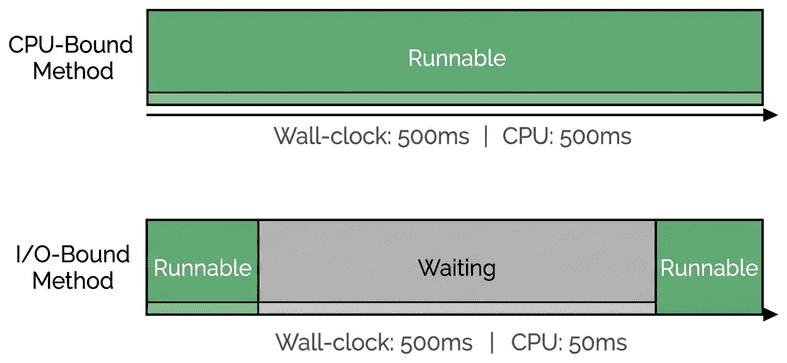
- High wall-clock time, high CPU time (CPU Bound): The method itself contains expensive computation. The thread stays Runnable throughout, and the CPU is doing the work.
- High wall-clock time, low CPU time (I/O Bound): The method is spending most of its time waiting. The CPU isn’t the bottleneck; something external is (I/O, network, lock contention).
In this lesson, we’ll focus on the CPU-bound case, where both metrics are high. This is the scenario where the Call Tree, combined with these metric pairs, gives us the most diagnostic power.
3.2. Inclusive Time vs. Exclusive Time
Regardless of whether we’re analyzing wall-clock time or CPU time, knowing that a method takes a long time still doesn’t tell us whether the method itself is slow, or whether it calls other methods that are slow. We need a way to separate the two:
- Inclusive time (also called total time) is the full time spent in a method, including the time spent in every method it calls, recursively.
- Exclusive time (also called self time) is only the time a method spends executing its own code, excluding time in child calls.
Let’s make this concrete with a simple example. Imagine three methods forming a call chain: methodA() calls methodB(), which calls methodC():
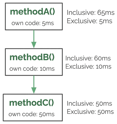
Let’s read this from the bottom up. methodC() runs 50ms of its own code and calls nothing else, so its inclusive and exclusive times are both 50ms. methodB() runs 10ms of its own code and then calls methodC(). Its exclusive time is 10ms (its own work), while its inclusive time is 60ms (10ms + the 50ms spent inside methodC()). The same pattern holds for methodA(): its exclusive time is just the 5ms it spends in its own code, while its inclusive time is the largest of the three because it accumulates the time of everything below it.
3.3. From Metrics to Diagnosis
When navigating a call chain top-down (as we’ll do in the Call Tree), a parent’s exclusive time is whatever remains after accounting for its children’s inclusive times. If methodA() shows 65ms inclusive and its only child shows 60ms inclusive, the parent’s own contribution is the remaining 5ms.
This gives us a diagnostic shortcut: a method with high inclusive time but low exclusive time is a pass-through that delegates work to its children. A method with high exclusive time is doing the expensive work itself. In our example, if we only saw methodA()‘s inclusive time of 65ms, we might blame it for the slowdown. The exclusive breakdown tells us the real story: methodA() contributes only 5ms of its own work, while methodC() is responsible for 50ms.
4. The Call Tree
The Call Tree is the view that brings both metric pairs together. It’s a cumulated representation of all method call stacks recorded during profiling, organized as a tree. Each node is a method, and its children are the methods it called.
Every node displays both inclusive and exclusive time, measured in either wall-clock or CPU terms. The tree is typically sorted by inclusive time, so the most expensive call path is always the first child at each level.
Let’s do a standard analysis workflow: start at the root (the entry point), then follow the heaviest path downward, always choosing the child with the highest inclusive time. At some point, the time shifts from inclusive to exclusive, meaning we’ve reached the node that’s doing the expensive work rather than passing it through:
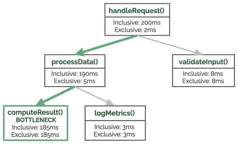
One important characteristic of the Call Tree is that it aggregates all invocations. If a method was called a thousand times, the tree shows its cumulative totals, not individual call timelines. This means a method that runs quickly once but is called millions of times can still show high totals in the tree, which is useful for spotting performance issues caused by excessive repetition rather than single slow calls. In algorithms with poor time complexity, this cumulative cost can balloon rapidly as input size grows. This is a hint that the bottleneck is algorithmic rather than incidental.
Now that we have the conceptual foundation, let’s see all of this in practice.
5. Analyzing Method Execution Time in JProfiler
With the conceptual foundation in place, let’s open JProfiler and apply what we’ve learned to the slow /campaigns/report endpoint.
5.1. Terminology Note
Before we begin, it’s worth noting that JProfiler uses slightly different terminology for the metrics we’ve discussed:
- Inclusive time → JProfiler labels this “Total Time”
- Exclusive time → JProfiler labels this “Self Time”
The underlying concepts are identical; only the labels differ.
5.2. Navigating to the Call Tree View
With an instrumentation profiling session active (as we learned in a previous lesson), we can find the Call Tree under the CPU Views section in JProfiler’s left panel. Make sure to use an instrumentation session; sampling mode does not report Self Time or invocation counts, so the column layout will look very different from what this lesson describes.
Before launching the service, it’s also a good idea to disable the workload simulator. With it running, the Call Tree aggregates all request types, making it much harder to isolate a specific endpoint. The simplest way to disable it is to comment out the @Component annotation on the simulator class before starting the application.
At the top of the Call Tree view, there’s a thread status selector. By default, it filters to Runnable, which effectively shows CPU time. Switching it to All states shows wall-clock time instead, since it includes periods when threads were waiting or blocked. For analyzing CPU-bound bottlenecks, the default Runnable filter is what we want.
To see all the columns used in this lesson, open View Settings and enable Show time, Show self time, Show invocations, and Show average times. These columns are not visible by default. The average time column is particularly important: it will later confirm that individual invocations are cheap, making the invocation count explosion the real diagnostic signal.
5.3. Checking a Healthy Endpoint
Before profiling, it’s a good practice to send a few warm-up requests to the application. A warm-up gives the JIT compiler time to optimize hot code paths (the code sections the JVM has detected as performance-critical). This ensures our measurements reflect steady-state behavior rather than one-time compilation overhead.
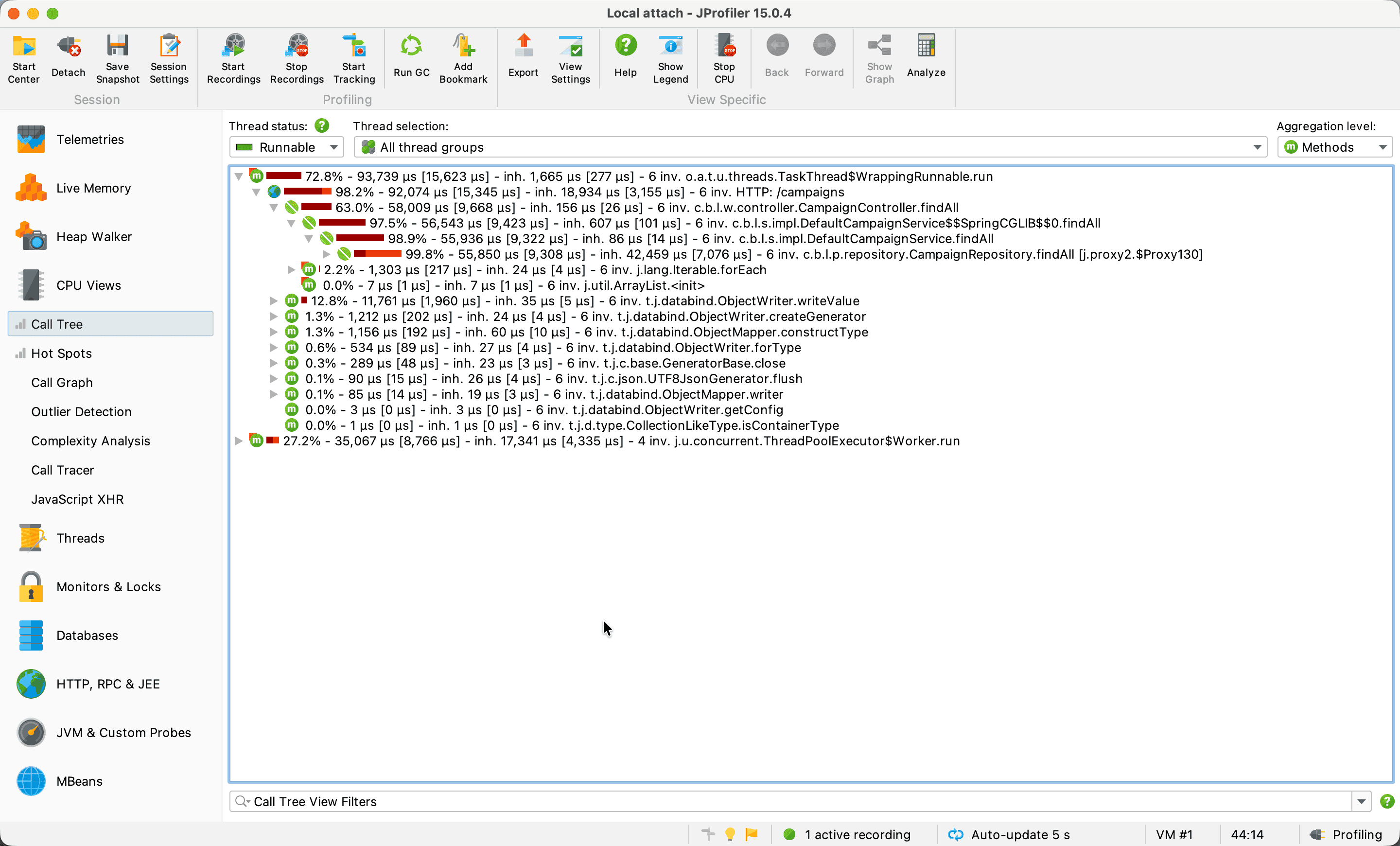
With the profiling session recording, let’s start by sending a request to a typical endpoint such as /campaigns. Opening the Call Tree, we can see a short, flat tree with small inclusive times. Each row in JProfiler uses this standard format:
<Percentage> - <Total Time> [<Avg Total Time>] - inh. <Self Time> [<Avg Self Time>] - <Invocations> inv. <Method Name>
The values in brackets are the per-invocation averages we enabled with the Show average times column in Section 5.2. Let’s see, for example, the line:
98.2% - 92,074 µs [15,345 µs] - inh. 18,934 µs [3,155 µs] - 6 inv. HTTP: /campaigns
Let’s see what a healthy endpoint looks like:
5.4. Profiling the Slow Endpoint
With the session still recording, let’s send a request to /campaigns/report and wait for the slow response. Opening the Call Tree, we can see a very different picture from the /campaigns baseline:
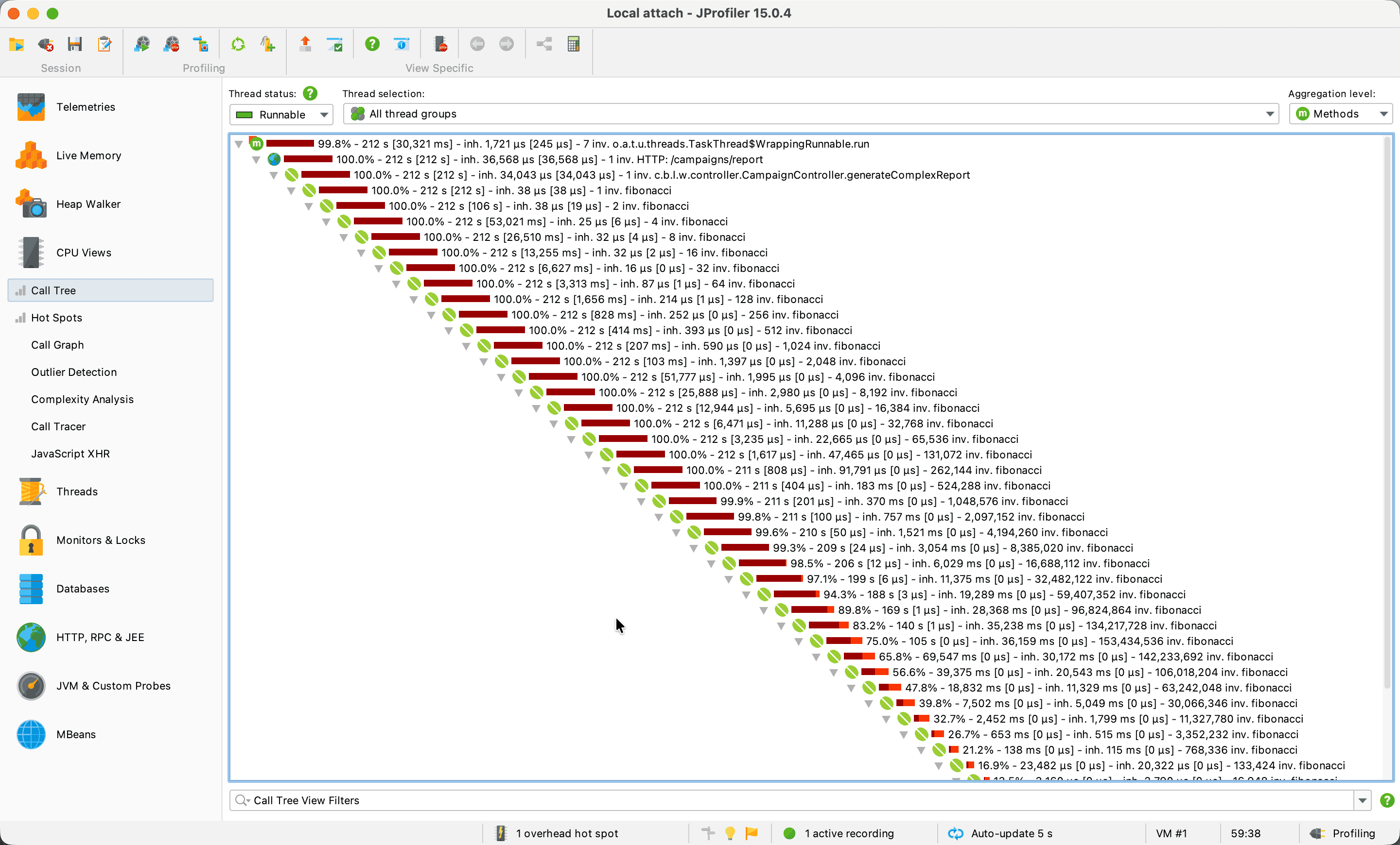
The primary diagnostic finding is the invocation count explosion: the number of fibonacci() invocations roughly doubles at each recursion depth level. This is the O(2ⁿ) complexity made visible in the Call Tree. The bug is not that any single call is slow (the average time column confirms each individual invocation is cheap), but that the naive recursive algorithm generates an exponential number of redundant calls.
The Self Time distribution tells the same story and connects directly back to the theory in Sections 3 and 4. Upper recursion levels show high Total Time but near-zero Self Time: each call just spawns two children and adds their results, passing all the work down. The deepest base-case levels have Self Time equal to Total Time: they have no further children, so all their time is their own work. Intermediate levels fall between the two extremes. No single call is doing expensive individual work; the cost is the cumulative sum of an enormous number of tiny invocations, which is exactly the aggregation pattern introduced in Section 4.
The bottleneck is algorithmic: the naive recursive implementation recomputes the same Fibonacci values exponentially, and that is what the Call Tree reveals.
Notice that for this particular bottleneck, wall-clock time and CPU time are nearly identical. The fibonacci() method is purely CPU-bound: the thread stays Runnable the entire time, doing computation without any waiting. If the bottleneck were I/O-related instead (such as a slow database query), we’d see a different pattern: high wall-clock time but low CPU time, because the thread would spend most of its time in a Waiting state. We could confirm this by switching the thread status selector from Runnable to All states and comparing the numbers. This is the diagnostic distinction from Section 3.1 in action.
The Call Tree showed us where the time is spent for a specific entry point. For a broader view that surfaces the most expensive methods across the entire application, regardless of entry point, we’ll explore the Hot Spots view in a future lesson.
6. Conclusion
In this lesson, we’ve explored three foundational concepts for analyzing method execution time.
Wall-clock time and CPU time measure different aspects of a method’s duration: the first counts everything including waiting, while the second counts only active computation. Inclusive and exclusive time tell us whether a method’s cost comes from its own code or from the methods it calls. The Call Tree combines both metric pairs into a navigable structure where we can trace a slow response to its root cause.
Using this approach on the java-profiling-app, we followed the heaviest path through the Call Tree and discovered that a recursive fibonacci() method was responsible for the slow /campaigns/report endpoint. This top-down, “follow the heaviest path” workflow applies to any performance investigation, not just the example shown here.