

Yes, we're now running our only Summer Sale. All Courses are 30% off until 20th July, 2026:
Learn through the super-clean Baeldung Pro experience:
>> Membership and Baeldung Pro.
No ads, dark-mode and 6 months free of IntelliJ Idea Ultimate to start with.
1. Introduction
In this tutorial, we’ll explore the Voronoi diagram. It’s a simple mathematical intricacy that often arises in nature, and can also be a very practical tool in science. It’s named after the famous Russian mathematician Georgy Voronoi. We can also refer to it as the Voronoi tesselation, Voronoi decomposition, or Voronoi partition.
Regardless of the name used, it’s hard not to recognize its pattern straight away since it has very unique visual characteristics. As such, we’re first going to gain some visual intuition. Then we’ll explore the mathematical rules behind it.
2. Definition
In the illustration below, we have a set of 40 randomly placed orange points on a 2-dimensional plane, along with its Voronoi diagram. The regions or tiles that we get as a result are called Voronoi cells:
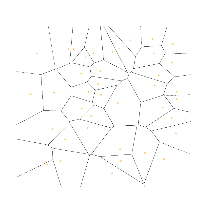
It’s immediately noticeable that most of the orange points are near the center of each cell. Every cell’s boundaries, however, are based on the distance to the points around it, and the black lines are drawn such that they divide the space between the points perfectly.
Furthermore, if we added any additional points inside a cell, they would be closest only to the cell’s original corresponding point. This means that the fewer points nearby, the bigger the resulting cell. In mathematical terms, we can concisely express the above-mentioned observations as follows:
For the given finite set of points  , each point,
  , has a corresponding Voronoi cell,
  , that consists of every point in the plane whose distance to is less than or equal to its distance to any other point from the set.
3. Computation
Now that we have a clear definition of what the Voronoi diagram is, we can set out to compute it. Many algorithms will do the job; however, the easiest one to understand actually requires us not to compute the Voronoi diagram directly, but rather to first compute the Delaunay triangulation of our set of points.
But what is the Delaunay triangulation exactly, and how does it help us with finding the Voronoi diagram? It’s a collection of triangles built using our original set of points as vertices. There is one condition though. No triangle’s vertex should lie inside the circumcircle of other triangles in the formation. For example, here’s an illustration of one such structure:
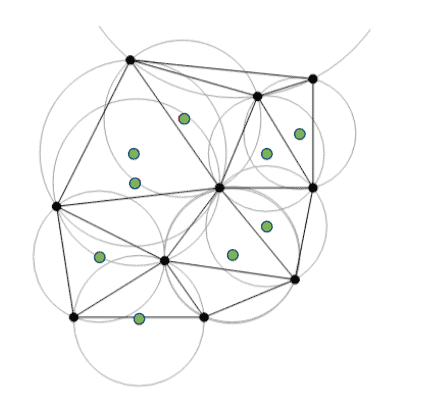
Here we have 10 points in black, and it’s easy to see that no other point lies within the drawn circumcircles. We also denote the origin of each circumcircle with a green dot, as it’s an important detail that will help us with finding the Voronoi diagram.
Let’s see why this is the case by comparing the Voronoi diagram at our first set of 40 points with its Delaunay triangulation side by side:
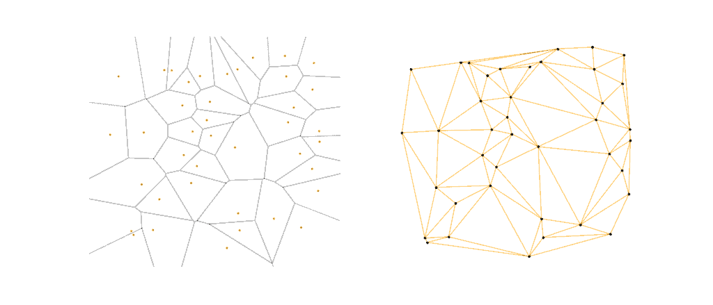
By closely comparing the two graphs visually, and imaging a circle around each triangle on the right, we can see a connection with the resulting Voronoi diagram on the left. Furthermore, every triangle circumcircle that we draw over actually corresponds to a vertex in the Voronoi graph.
That is why if we have a ready Delaunay triangulation, we just need to find the edges of our Voronoi graph by forming an edge from each neighboring triangle’s circumcenter to its own circumcenter. Pretty neat!
So how do we go about calculating the Delaunay triangulation then? One way to do it is using the Bowyer-Watson algorithm.
This algorithm works by iteratively adding points to an existing Delaunay triangulation, usually starting from a very simple triangulation, like one that encloses all the points to be triangulated. After every insertion, we check if any triangles’ circumcircles contain the new point, and if so, we delete them, leaving a cavity and then joining the vertices on the cavity boundaries.
The pseudo-code for a basic implementation is actually pretty straightforward:
algorithm BowyerWatson(pointList):
    // INPUT
    //    pointList = a list of points to be triangulated
    // OUTPUT
    //    The triangleList with the Delaunay triangulation of the points

    Create a super triangle that surrounds all the points
    Add the super triangle to the triangle list

    for point in pointList:
        edgeList <- an empty set

        for triangle in triangleList:
            if point is within the circumcircle of triangle:
                set triangle as incorrect
                add edges of triangle to edgeList

        Remove all incorrect triangles from triangleList

        for edge in edgeList:
            if edge is shared by any other triangles:
                remove edge from edgeList

        for edge in edgeList:
            form a triangle from edge to point
            add triangle to triangleList

    for triangle in triangleList:
        if triangle contains a vertex from the super triangle:
            remove triangle from triangleList

    return triangleList
The computation complexity of this algorithm can be improved further by careful choice of data structure, but this exact formulation checks all the triangles for connectivity, and therefore amounts to  .
.
4. Conclusion
In this brief article, we visually introduced the intricate Voronoi diagram alongside its closely related cousin, the Delaunay triangulation. Using their found relationship, we encouraged the use of the Bowyer-Watson algorithm by explaining how it can help calculate the final diagram.