Learn through the super-clean Baeldung Pro experience:
>> Membership and Baeldung Pro.
No ads, dark-mode and 6 months free of IntelliJ Idea Ultimate to start with.
Last updated: February 13, 2025

Learn through the super-clean Baeldung Pro experience:
>> Membership and Baeldung Pro.
No ads, dark-mode and 6 months free of IntelliJ Idea Ultimate to start with.
Autoencoders are a powerful deep learning methodology. They’re chiefly used for pre-training and generative modeling, though, they have other uses as well. The basic autoencoder trains two distinct modules known as the encoder and the decoder respectively. These modules learn data-encoding and data-decoding respectively. The variational autoencoder offers an extension that improves the properties of the learned representation and the reparameterization trick is crucial to implementing this improvement.
In this article, we’ll explain the reparameterization trick, why we need it, how to implement it and why it works. We first provide a quick refresher on variational autoencoders (VAEs). We then explain why the VAE needs the reparameterization trick, what the trick is and how to implement it. After explaining the use of the trick we justify it formally.
VAEs are popular and fundamental unsupervised learning architectures for neural network-based models. VAEs improve on the vanilla autoencoder by creating more continuous embedding spaces.
An autoencoder consists of two neural network modules. One module, the encoder, takes the input data and projects it to another vector in a new embedding space. The second module, the decoder, takes this vector and converts it back to the original input. We train the model by minimizing the difference between the original input and the reconstructed output. This basic format is referred to as the vanilla autoencoder.
This works very well and many images can be reconstructed correctly. In this paradigm, the decoder serves as a generative model. Given a sample from the encoding space we should be able to generate a reasonable image that may exist, even if we have never seen this exact image that leads to this encoding before.
Unfortunately, for vanilla autoencoders, this is not the case and linear samples between two encodings do not lead to good generated samples. This is because there are discontinuities in the embedding space that don’t lead to smooth transitions.
We provide an example of this phenomenon here. For a 2-dimensional embedding, we see the transition between a  and a
and a  . We do this by linearly interpolating along each dimension. In this way, the x-axis is the linear interpolation between the first element of the vector embedding and the first element of the vector embedding.
Similarly, the y-axis is the linear interpolation between the second, and last since we use a 2-d embedding, element of the vector embedding and the second element of the vector embedding:
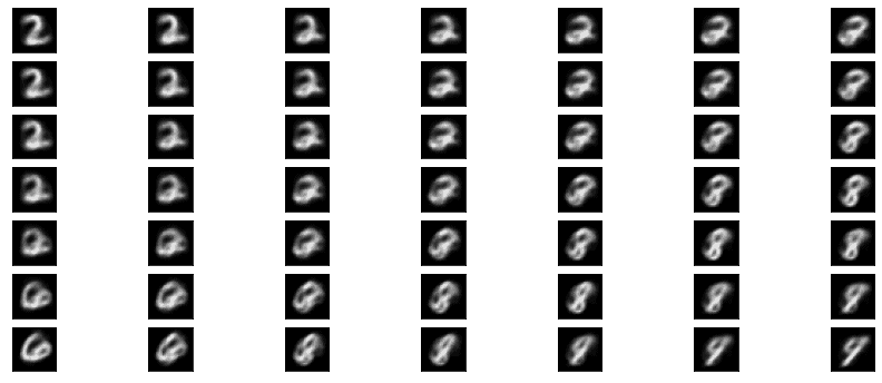
The lack of form the reproductions have in between the extremes is clearly visible. The VAE will help to alleviate this issue.
A VAE differs from a vanilla autoencoder in how it treats the learned Representation. It was proposed in a paper by Dietrich Kingma and Max Welling.
A VAE learns the parameters of a gaussian distribution:  and its standard deviation
  . These are then used to sample from a parameterized distribution:
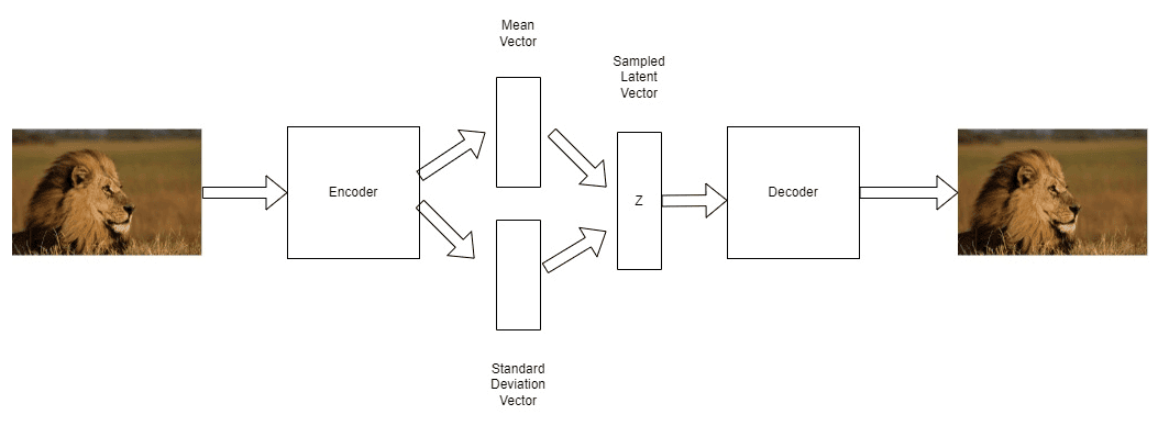
In the above image, we can see this process. The encoder learns to predict two vectors, the mean and standard deviation of a distribution. These are then used to parameterize the distribution and generate a sample,  . is then decoded using the learned decoder.
The VAE predicts the parameters of a distribution which then is used to generate encoded embeddings. This process of sampling from a distribution that is parameterized by our model is not differentiable. If something is not differentiable that is a problem, at least for gradient-based approaches like ours. So we need some method of making our predictions separate from the stochastic sampling element.
We can solve this problem by applying the reparameterization trick to our embedding function. What does that mean? It means rewriting our implementation of how we parameterize our Gaussian sampling. We now treat random sampling as a noise term.
In the case of a Gaussian distribution, we treat our noise as a standard normal distribution. That is, a Gaussian that has a mean  and a variance of
  . This noise term is now independent of and not parameterized by our model.
A nice property of the Gaussian is that to change the mean and variance of a sample we can simply add the mean and multiply by the variance. This has the effect of scaling a sample from our noise distribution. The benefit is the prediction of mean and variance is now no longer tied to the stochastic sampling operation. This means that we can now differentiate with respect to our models’ parameters again.
We visualize our model and show how it is changed by reparameterization in the diagram shown. When is sampled stochastically from a parameterized distribution we see that all our gradients would have to flow through the stochastic node. In contrast, reparameterization allows a gradient path through a non-stochastic node. We relegate the random sampling to a noise vector which effectively separates it from the gradient flow:

By using this intuition, we can effectively implement the VAE.
Previously our model  predicted the parameters of a gaussian distribution which we instantiated and then sampled from. Now, we take advantage of a neat property of a gaussian which allows us to sample from the standard normal distribution. The standard normal is a Gaussian distribution with mean,
 , and standard deviation,
 .
.
This Gaussian sample can then be scaled by our predicted mean and variance. We now have samples drawn from a fixed Gaussian distribution, which we add our to and multiply by our standard deviation :
(1) 
This approach uses a fixed source of noise,  which we sample from. Generally, we’ll treat as a sample from a Normal distribution. We can see how this approach differs by examining our new diagram.
We have now separated our random element from the learned parameterization and we can now differentiate through our model again. In the following section, we take a deeper look at the math behind these ideas and justify our approach.
We can now take a deeper look at why this approach works and allows us to differentiate through the stochastic sampling our model needs to do.
We’re interested in taking the derivative of our parameterized Gaussian:
(2) ![\begin{equation*} \triangledown_{\theta}\mathbb{E}_{x \sim p_{\theta}(x)}[f(x)] \end{equation*}](/wp-content/ql-cache/quicklatex.com-b0bef21f672b58390cc7b3a82d72564c_l3.svg "Rendered by QuickLaTeX.com")
The issue we have is that the gradient is being taken with regard to a stochastic quantity, the distribution  parameterized by
  . We can’t take the gradient of a stochastic quantity so we need to rewrite it. Below, we introduce some new representations as follows:
(3) 
We represent as a sample from a distribution. This is a source of noise and stochasticity.
(4) 
We write  our embedding vector as a parameterized function of our noise . In equation 5 we see how the two expressions are equivalent but how we have moved the stochasticity out of . The derivative of this function is now separate from the noise and we rewrite our expression to move the expectation outside of the derivative:
(5) ![\begin{equation*} \begin{aligned} \triangledown_{\theta}\mathbb{E}_{x \sim p_{\theta}(x)}[f(x)] &= \triangledown_{\theta}\mathbb{E}_{\epsilon \sim q(\epsilon)}[f(g_{\theta}(\epsilon))]\\ &= \mathbb{E}_{\epsilon \sim q(\epsilon)}[\triangledown_{\theta}f(g_{\theta}(\epsilon))] \end{aligned} \end{equation*}](/wp-content/ql-cache/quicklatex.com-cb27b34ec0803a9f77ffd0dcc568047e_l3.svg "Rendered by QuickLaTeX.com")
We link this back to what we had in 1. This is our function  . Where the and are our learned predictions for an input . We have pushed the stochasticity out of our learned function and we can now differentiate through it with respect to .
Variational autoencoders are a powerful unsupervised learning architecture. The reparameterization trick is a powerful engineering trick. We have seen how it works and why it is useful for the VAE. We also justified its use mathematically and developed a deeper understanding on top of our intuition.
Autoencoders, more generally, is an important topic in machine learning. As a generative model, they have myriad important uses and this helps to explain their long-lived popularity.