

Learn through the super-clean Baeldung Pro experience:
>> Membership and Baeldung Pro.
No ads, dark-mode and 6 months free of IntelliJ Idea Ultimate to start with.
Learn through the super-clean Baeldung Pro experience:
>> Membership and Baeldung Pro.
No ads, dark-mode and 6 months free of IntelliJ Idea Ultimate to start with.
In this tutorial, we’re going to have a look at Timsort. This is a comparatively recent sorting algorithm – developed in 2002 by Tim Peters for the Python programming language but now used much more widely.
Timsort is a sorting algorithm developed by Tim Peters in 2002. It was originally developed for use in Python and is now the standard sorting algorithm that the Python standard library uses. It’s also used in other languages. For example, Java uses it as the standard sorting algorithm for arrays of non-primitive values.
Timsort has been developed to work well on real-world data. In particular, it takes advantage of “natural runs” of data within the entire collection. These are parts of the collection that are already considered to be in order, even if the entire collection might not be. It works as a hybrid between Merge Sort and Insertion Sort. It’s considered to be a stable sorting algorithm – that is, elements of equal value in the original collection will remain in the same order in the final collection.
The main Timsort algorithm consists of three phases – we calculate a run length, sort each run of elements using insertion sort, and then recursively sort adjacent runs using merge sort:
algorithm Timsort(array):
    // INPUT
    //    array = the unsorted collection
    // OUTPUT
    //    the sorted collection

    // Calculate run length
    runLength <- calculateRunLength(array)

    // Perform insertion sort on each run
    for start <- 0 to array.length by runLength:
        end <- min(array.length - 1, start + runLength - 1)
        insertionSort(array, start, end)

    // Recursively merge adjacent runs
    mergeSize <- runLength
    while mergeSize < array.length:
        for left <- 0 to array.length by mergeSize * 2:
            mid <- left + mergeSize - 1
            right <- min(array.length - 1, left + (2 * mergeSize) - 1)
            if mid < right:
                merge(array, left, mid, right)
mergeSize <- mergeSize * 2The exact way that the run lengths are determined isn’t important. What’s important is the details of what the run length is.
Insertion sort is most efficient on short collections, so we want our run length to be relatively small. At the same time, the merging algorithm works best when the number of runs is a power of two or slightly less than one. We also want to minimize our number of runs, preferring slightly longer runs over more of them, as long as they don’t get too long.
One such algorithm for this involves starting with the entire array length and halving it until we get below a certain threshold. By halving it each time, we guarantee that we’ll have a power of two for the number of runs. Equally, our threshold will mean that we keep the number of runs down to a minimum that is still efficient enough for the insertion sort portion:
algorithm DeterminingRunLength(array):
    // INPUT
    //    array = input collection
    // OUTPUT
    //    Run Length

    runLength <- array.length
    remainder <- 0

    while runLength > THRESHOLD:
        if isOdd(runLength):
            remainder <- 1
        runLength <- floor(runLength / 2)

    return runLength + remainder
For example, if we have an array of length 19 and a threshold of 8 then we’ll get:
 = 1,
= 1,  = 9 = 1, = 4
And so, our calculated run length will be 5. This means we’ll have 4 runs, the first three of length 5 and the last one of the remaining 4 elements.
One interesting side effect of this is that if the original collection is shorter than our threshold, we’ll generate only a single run. This then means that we’ll drop out to an insertion sort instead, which will likely be more efficient than also doing the merges for such a short collection.
Now we know what length we want our runs to be, we start by using insertion sort on each run individually. Insertion sort is a good choice here because it’s efficient on relatively short collections:
algorithm InsertionSort(array, left, right):
    // INPUT
    //    array = the input collection
    //    left = the left index
    //    right = the right index
    // OUTPUT
    //    array is sorted between left and right indices

    for index <- left + 1 to right:
        temp <- array[index]
        index2 <- index - 1
        while index2 >= left and array[index2] > temp:
            array[index2 + 1] <- array[index2]
            index2 <- index2 - 1
        array[index2 + 1] <- temp
This is just a standard insertion sort algorithm. We iterate over our run and shift any elements to the left until they’re in the right position.
Once we have a collection of runs that are internally sorted, we can begin to merge them together. This uses the merging algorithm that merge sort uses, but because the runs are already sorted, we only need the merging part.
We start out by merging adjacent runs together. After this, we’ll have effectively got sorted runs that are twice the length of before. We can keep recursively merging these growing runs together until we’ve merged the entire collection.
The merging of two runs together works by iterating over both runs at the same time and, at each step, selecting the lowest element from the two. When we reach the end of one of the runs, we can select everything remaining from the other run – since we know that they must all be greater than the last selected element:
algorithm MergingRuns(input, left, mid, right):
    // INPUT
    //    input = the input collection
    //    left = the left index
    //    mid = the mid index
    //    right = the right index
    // OUTPUT
    //    The sorted collection resulting from merging the subarrays

    leftArray <- input[left : mid]
    rightArray <- input[mid + 1 : right]

    leftIndex <- 0
    rightIndex <- 0

    while leftIndex < len(leftArray) and rightIndex < len(rightArray):
        leftValue <- leftArray[leftIndex]
        rightValue <- rightArray[rightIndex]

        if leftValue < rightValue:
            input[left + leftIndex + rightIndex] <- leftValue
            leftIndex <- leftIndex + 1
        else:
            input[left + leftIndex + rightIndex] <- rightValue
            rightIndex <- rightIndex + 1

    for leftIndex <- leftIndex to length(leftArray) - 1:
        input[left + leftIndex + rightIndex] <- leftArray[leftIndex]

    for rightIndex <- rightIndex to length(rightArray) - 1:
        input[left + leftIndex + rightIndex] <- rightArray[rightIndex]
Once we’ve done this for every pair of runs, we can simply repeat it for the new sets of longer runs until we have nothing left to do.
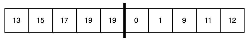
This all seems very complicated, so let’s instead look at a real example of it in action. For this, we’re going to sort the following set of numbers:

The first step is to determine our run length. We’ll have a threshold of 8, which gives us a run length of 5 elements and, therefore 4 runs:

Next, we’ll perform the insertion sort on each of these runs:

We’re now ready to start merging our runs together. The first thing we’ll do is merge runs #1 and #2 together, and runs #3 and #4 together:

Finally, we merge the remaining two runs together:

And now we have a fully sorted collection.
We already have an algorithm that’s pretty efficient, but there are a few things that we can do to tweak it and make it even more so in certain circumstances.
We’ve already seen how the merge algorithm will reach the end of one run of numbers and immediately add all other runs onto the end. We can do this because we know that both runs are already in order within themselves, so if we’ve run out of one run, we know that the other must belong at the end.
We can go further than this, though. Sometimes, we may have a situation where one entire run belongs after the other. For example, if we were merging the following two runs:
If we follow the simple merge algorithm, we’ll compare each of the numbers in the right run to the first number in the left run. Then when we get to the end of them, we’ll add all of the left runs to the end. This works, but it means we’ve had to perform 5 comparisons to get there.
Instead, if we compare the last number of the right run to the first number of the left run, then we can immediately tell what the end result should be without needing all of those comparisons.
This means that in two comparisons – one for the start of each run to the end of the other one – we can detect if one entire run belongs before the other entire run. If this is the case, we can immediately do the merge with no extra work. This is especially beneficial if our runs are longer. For example, if our runs were 30 items long, then we can potentially sort it all in 1 or 2 comparisons.
Another trick that we can use is to do our insertion sorts over more than one run at a time. For example, we can do it over pairs of adjacent runs. As long as our runs are short enough, this is still relatively efficient, and it’ll help get more elements already into order and so make the merging more efficient. For example, this will mean that galloping is more likely to happen because adjacent runs are already in order.
For example, if we do this for our above example, then our values after the insertion sorts will be:

For this, we did our insertion sort across runs #1 and #2 and also across runs #3 and #4. Immediately we can see that our first pass of merges will be galloping because these adjacent runs are sorted across them.
We can also do the insertion sorts so that they overlap. For example, if we do the insertion sorts across runs #1 and #2, then across #2 and #3, and finally across #3 and #4 then we get this:

This gives us less galloping – runs #1 and #2 aren’t in strict order. But it does mean that all of run #1 fits into the middle of #2, and it’ll mean that the next round of merging may be more efficient as well.
The worst possible case for insertion sort is when the run is in strict reverse order. However, we can detect this and handle it as a special case. If our data is likely to contain runs like this, then we can look for it and, in that case, reverse the run instead of doing a real sort.
We can even go further than this and detect reverse-ordered subsections of the run instead. If we do this, then we’d still need to sort it afterwards, but the sorting will be much more efficient because the list is already much closer to the correct order.
For example, given the following run:
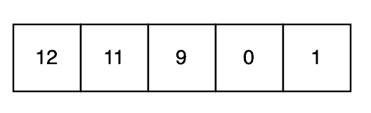
This is almost the worst case for insertion sort – because almost every number is in the wrong position, and almost every number has the maximum possible distance to move. However, we can detect that the subsequence 12-11-9-0 is in strict reverse order and handle that case first:
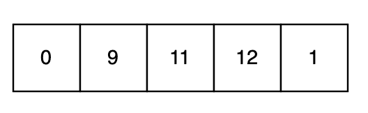
All of a sudden, we’re in a much better position. We now only need to move a single number into the correct position and the entire run is sorted.
We can even detect that it was the start of the collection that we reversed and skipped over it for the insertion sort, meaning that we’ll immediately start on the “1” and shift it into position.
We saw earlier that if the entire collection was shorter than our run length threshold, the algorithm would degrade into just doing a single insertion sort. This is desirable because insertion sort is very efficient for short collections.
However, we can do even better than that. If we have a known upper limit that we’re happy to only do an insertion sort with, we can check if the incoming collection is shorter than that and degrade immediately. This known limit can be longer than our run length threshold as well to help give more ideal runs in the case that we’re going to do the full Timsort algorithm.
For example, we might decide to have a run length threshold of 8, but we’re happily degrading to insertion sort for any collection that is 32 items or less. This means that it’s only for collections larger than this that we’ll ever do the extra work.
Timsort works by splitting the collection into pieces of work and then working on each one independently of the others. This means that we can parallelize this work to a great extent. For example, we can do all of the insertion sorts on all of the runs simultaneously in parallel instead of doing them sequentially.
This won’t make the algorithm more efficient, but it’ll reduce the wall time that it takes to complete.
Here we’ve seen Timsort, including how the algorithm works and some optimisations that can be leveraged to make it even more efficient. As with all sorting algorithms, the data and exact requirements are important to determine the best sorting algorithm to use, but why not consider Timsort next time you need to select one?