

1. Introduction
In this article, we’ll learn what red-black trees are and why they’re such a popular data structure.
We’ll start by looking at binary search trees and 2-3 trees. From here, we’ll see how red-black trees can be considered as a different representation of balanced 2-3 trees.
The aim of this article is to explain red-black trees in a simple way, so we won’t delve into code examples or detailed examples for all possible cases of insertion and deletion.
2. Binary Search Trees
A binary search tree (BST) is a tree where every node has 0, 1, or 2 child nodes. Nodes with no child nodes are called leaves. Furthermore, the value of the left child of a node must be smaller than the value of the node, and the value of the right child must be bigger than the value of the node.
Let’s start with a simple example:
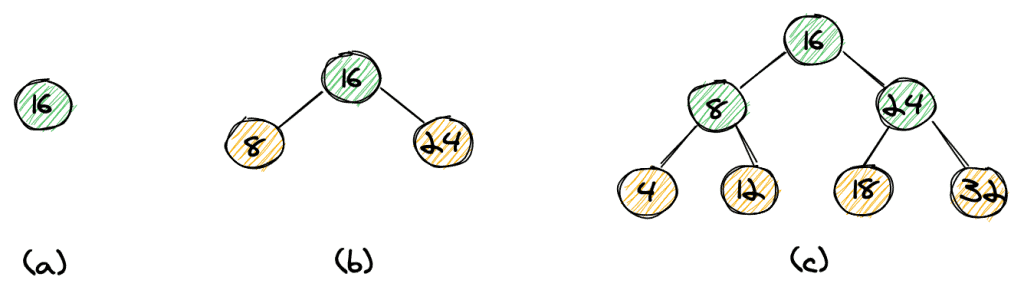
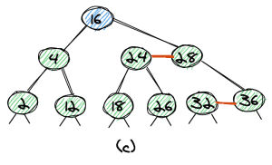
We have the elements 4, 8, 12, 16, 18, 24, 32. We can start our tree with element 16 as the root (a), then insert 8 and 24 (b), and eventually insert the elements 4, 12, 18, and 32 (c). Notice how the left child is always smaller than its parent and the right child is always bigger than its parent. We can easily see that the height of the tree is log n, with n being the number of elements.
If we want to search an element in our tree, we can start off at the root. If the element we are looking for is equal to the root, we’re done. In case it’s smaller, we continue our search to the left, and in case it’s bigger, we continue to the right. We continue until we have found the element, or until we’ve reached a leaf-node (in yellow). It’s quite straightforward to see that the time complexity for our search would be O(log n).
However, the structure of the tree highly depends on the order in which elements are inserted. If we insert elements in order 24, 32, 16, 18, 12, 8, 4, the resulting tree isn’t balanced anymore (d). If we insert elements in sorted order, the result is a tree with only one child per node (e). That’s actually a list, not a tree. That means that our worst-case complexity to find and an element is O(n).
3. Balanced 2-3 Trees
3.1. Definition of a 2-3 Tree
We’ll now look at 2-3 trees, which help us to maintain a balanced tree, no matter in which order we insert elements into our tree. A 2-3 tree is a tree with two types of nodes. A 2-node has one value and two child nodes (again, the left child has a smaller value and the right child has a bigger value), and a 3-node has two values and three child nodes.
The left child of a 3-node is smaller than the left value of the parent. The middle child’s value is in between the two parent values, and the right child’s value is bigger than the parent’s right value.
3.2. Inserting Elements Into a 2-3 Tree
Let’s see how to insert the elements 32, 24, 18, 16, 12, 8, 4 into a 2-3 tree while keeping the tree balanced.
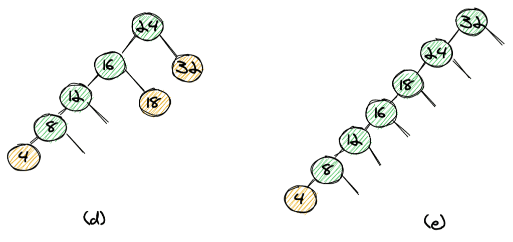
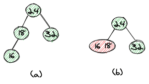
We start off with 32, which gives us a tree with only the root node (a). We then insert 24 which gives us a 3-node at the root (b).
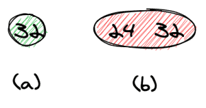
Next, we’ll insert the next element, 18, as a left child of the root (as 18 is smaller than 24). This leads to an unbalanced tree. We can get a balanced tree by moving the 24 out of the 3-node and making it the root node.
The result will be a balanced tree with only 2-nodes (b).
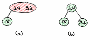
The next element we want to insert is 16. Again, we end with an unbalanced tree (a). This time we can simply move the 16 one level up to form a 3-node together with 18 (b).
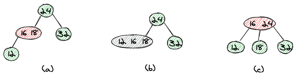
Next, we insert 12 as a left child of the 3-node we just created (a). To balance the tree, we first move the 12 one level up to form a temporary 4-node (b).
We can now split up the 4-node by moving the middle element, 16, to the root, which again gives us a nicely balanced tree (c).
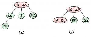
The insertion of 8 is now quite straightforward — we first create a left child of 12 (a) and then move the element one level up to form a 3-node with 12 (b).
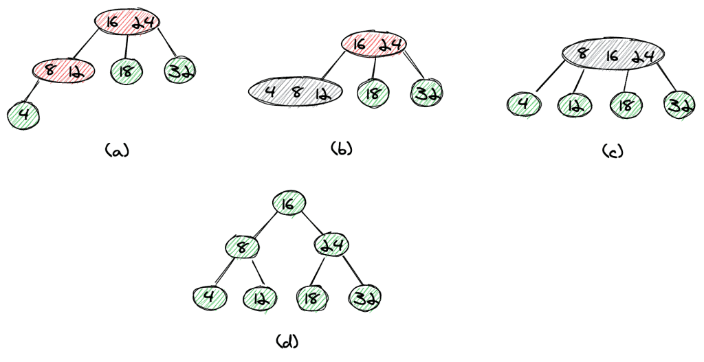
The last element to insert, 4, leads to a slightly more complex insertion. First, we create a left (a) and move it one level up which gives us a temporary 4-node (b). Now we can move the middle element, 8, one level up to get a 4-node at the root (c).
In the last step, we split up the 4-node by extracting 16 as the root node (d).
3.3. Complexity of Insertion
The above example shows that it’s possible to insert elements in such a way that we maintain a balanced tree. However, the operations to perform for every insertion are quite complex to express in code. The reason is that we need to have three different types of nodes (2-nodes, 3-nodes, and 4-nodes).
Furthermore, we need to distinguish several different cases in order to move elements up to and merge into 3-nodes or split 3-nodes into 2-nodes.
In the next section, we’ll see how red-black trees can help us to reduce this complexity.
4. Red-Black Trees
4.1. Correspondence With 2-3 Trees
A red-black tree is essentially a different representation of a 2-3 tree. Let’s dive directly into an example:
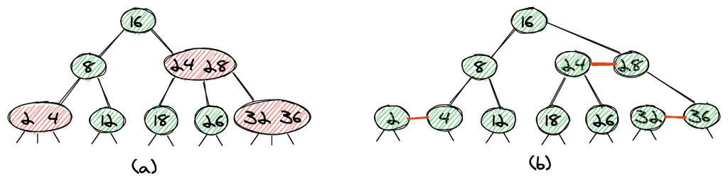
The tree in (a) shows a 2-3 tree as we’ve seen it in the previous section. We have marked the 3-nodes in red, which leads us directly to a red-black tree. We split every 3-node into two 2-nodes and mark the link between the two in red.
This also directly leads us to two of the main properties of red-black trees:
- A red link is always followed by two black links (because the 3-node we split is followed by three black links).
- The path from the root to a leaf-node always contains the same number of black links (this follows directly from the fact that our 2-3 tree is balanced).
On top of that, we add the following two conditions:
- Only links to the left child (the smaller child node) can be red. This condition simplifies the implementation even more.
- All leaves have null links (nil).
4.2. Why This Representation?
In short, it simplifies the implementation of the tree and the operations. We can use the same operations as for a binary tree (for example, finding a value works exactly the same way as in a “normal” binary tree).
4.3. Insertion
To insert a new value into a red-black tree, we add a new node as a new leaf-node. This, of course, leads to an unbalanced tree. To balance the tree, we first color the link to our new node in red.
We then need only three kinds of operations to rebalance our tree. Let’s have a look at these operations.
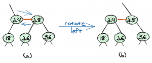
The first operation is the left rotation. Here, we transform the sub-tree (a) into sub-tree (b) by moving two links.
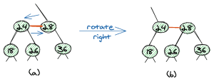
The second operation is the right rotation, which is the exact opposite of the left rotation.
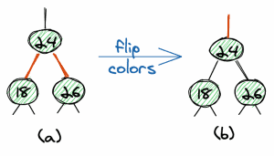
The third operation is a flip of colors. We can change two red links into two black links and change the parent link into a red link.
The important thing here is that all three operations are local operations, which means they do not have an effect on the whole tree.
In this article, we won’t look at a full example of an insertion. The main point to underline here is these three simple operations allow us to easily rebalance the tree.
4.4. Example of an Insertion
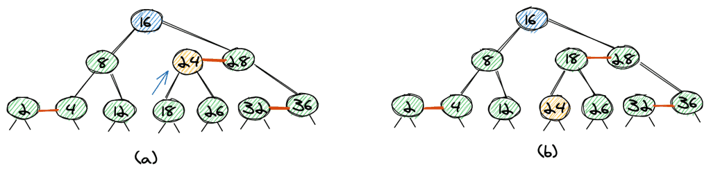
Let’s look at an example of an insertion of an element into a red-black tree. The element we want to insert is 37 (orange background) and the root is shown with a blue background.
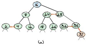
First, we start at the root and walk down the tree until we have found the leaf-node where to insert the element. In our case, 37 will be the biggest element in the tree, so it’s on the very right. The link to the new node is red, and we get a tree as shown in (a).
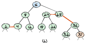
Since the parent element 36 now has two red links, the second step is the flip-colors operation, which leads us to the tree as shown in (b).
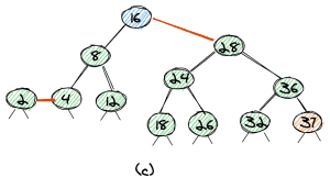
As now the node with value 28 has two red links, the third step is a flip-colors operation again, which leads to the tree as shown in (c).
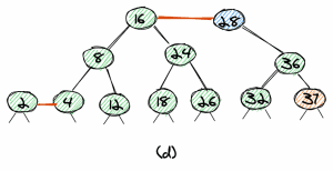
As we want all our red links to lean left, we do a left-rotation, which leads to the tree in (d), with 28 as the root. We can easily see that the tree is balanced.
4.5. Deletion
We can use the same three operations to rebalance the tree after we’ve deleted a node. In this article, we won’t look at a full implementation, but only outline the idea and give a few examples of deleting an element.
For all examples, we’ll start off with the following (valid) red-black tree:
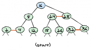
The trivial case is the deletion of a leaf-node with a red link. Let’s look at the two possible cases, deleting 2 and 36.
Delete 2
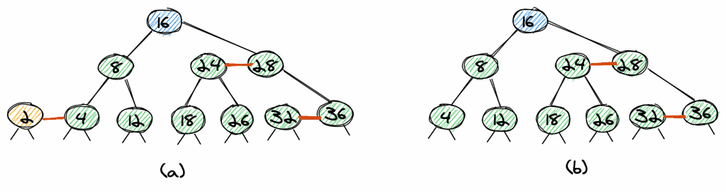
That’s the easiest case. The element 2 is the left node of a red link, so we can delete it and directly get a valid red-black tree without any need for rebalancing.
Delete 36
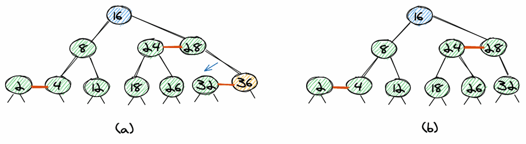
If we want to delete 36, we again remove the node, however, as 36 is the right node of the red link, we need to change the link from 28 to 36 to point to 32. Again, we get a valid red-black tree.
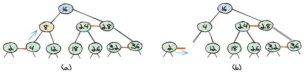
Delete 8
If we want to delete a non-leaf node, we can first make it a leaf-node. To do so, we find the maximum element of the left subtree or the minimum element of the right subtree. This exchange does not change the red-black tree property. Because we can move every node to the bottom of the tree, it’s sufficient to understand how to delete leaf-nodes.
Let’s look at how to delete the element 8. The maximum value of the left subtree is 4 (a). So we exchange nodes 8 and 4 and remove it. As the 8 had a red link, we have the same trivial case as if we removed element 4 (b).
Again, the final tree is a valid red-black tree (c).
Delete 24
Things become a little more complicated if we want to remove a leaf-node which is not the right or left node of a red link.
As an example, let’s look at the deletion of 24 (a). First, we flip 24, and 18 (18 is the maximum element of the left subtree).
We now need to remove 24 in the tree (b), which has no red link.
The tree with 24 removed (c) is not a valid red-black tree as 18 has only one child, so the tree isn’t balanced.
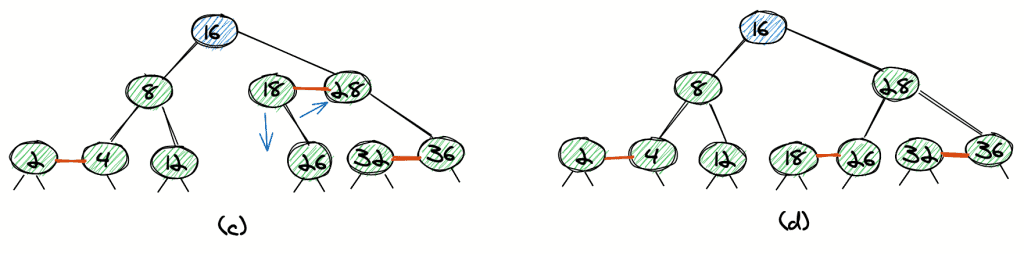
We can balance the tree with a rotation (d).
5. Complexity
Red-black trees offer logarithmic average and worst-case time complexity for insertion, search, and deletion.
Rebalancing has an average time complexity of O(1) and worst-case complexity of O(log n).
Furthermore, red-black trees have interesting properties when it comes to bulk and parallel operations. For example, it’s possible to build up a red-black tree from a sorted list with time complexity O(log(log n)) and (n/log(log n)) processors.
6. Applications of Red-Black Trees
Real-world uses of red-black trees include TreeSet, TreeMap, and Hashmap in the Java Collections Library. Also, the Completely Fair Scheduler in the Linux kernel uses this data structure. Linux also uses red-black trees in the mmap and munmap operations for file/memory mapping.
Furthermore, red-black trees are used for geometric range searches, k-means clustering, and text-mining.
From the above example, we can see that red-black trees are mainly used under-the-hood, and we, as developers, don’t come into contact with them that often, even though we use them on a daily basis.
7. Conclusion
In this article, we learned what red-black trees are and how they are basically a different representation of the 2-3 trees.
We also saw a table that summarizes the complexity of operations on the tree, and eventually, we shortly summarized some real-world applications of red-black trees.
However, when it comes to the selection of a data structure for a specific use case, there are many factors to consider. Red-black trees are especially useful if we require good average cost for insertion and search, as well as guaranteed logarithmic worst-case costs for these two operations.
Furthermore, red-black trees are a good choice if we have frequent updates to our tree, as the rebalancing costs are lower than for other balanced trees like AVL or B-trees, for example.