Recurrent Neural Networks

1. Overview

In this tutorial, we’ll talk about Recurrent Neural Networks (RNNs), which are one of the most successful architectures for processing sequential data. First, we’ll describe their basic architecture and differences from traditional feedforward neural networks. Then, we’ll present some types of RNNs, and finally, we’ll move into their applications.

2. Basic Architecture

First, let’s discuss the basic architecture of an RNN to get a deeper knowledge of why these networks perform so well on sequential data.

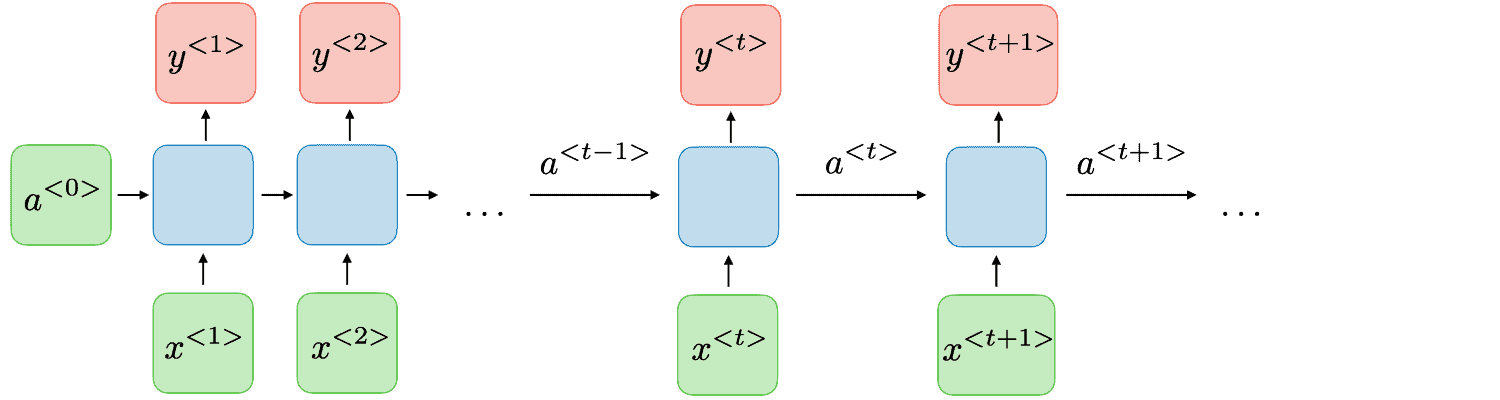
Every RNN consists of a series of repeating modules that are called cells and process the input data sequentially. That means that the first cell takes as input the first sample of the sequence, the second cell takes the second sample, and so on. Each cell takes the input vector and, after some processing, generates a vector known as a hidden state that is passed to the next cell . That means that each time the hidden state captures all the information given so far, enabling the network to have some memory.

In the image below, we can see a basic diagram that illustrates the basic architecture of an RNN:

We can build an RNN in Python using TensorFlow or PyTorch. The following codes give an example of how to build a classifier using RNN in TensorFlow:

import tensorflow as tf

class RNNModel(tf.keras.Model):
    def __init__(self, units, input_feature_dim, num_classes):
        super(RNNModel, self).__init__()
        # The first RNN layer
        self.rnn_layer_1 = tf.keras.layers.SimpleRNN(units, return_sequences=True, input_shape=(None, input_feature_dim))
        # The second RNN layer
        self.rnn_layer2 = tf.keras.layers.SimpleRNN(units, return_sequences=False)
        # Full connected layer
        self.fc = tf.keras.layers.Dense(num_classes)
        
    def call(self, inputs):
        x = self.rnn_layer(inputs)
        output = self.fc(x)
        return output

# Hyperparameters
input_feature_dim = 10 # Number of features
units = 20 # Number of units in RNN cell
num_classes = 3 # Number of output classes

model = RNNModel(units, input_feature_dim, num_classes)

In this example, input_shape is defined as (None, input_feature_dim), where None stands for an unspecified number of timesteps. It allows for variable sequence lengths. When there are multiple layers in the RNN, we set return_sequences=True for all the layers apart from the last one. By setting return_sequences=True, the network passes the sequence of outputs to the next layer.

We can also build the same classifier using PyTorch:

import torch
import torch.nn as nn

class RNNModel(nn.Module):
    def __init__(self, input_size, hidden_size, num_layers, num_classes):
        super(RNNModel, self).__init__()
        self.hidden_size = hidden_size
        self.num_layers = num_layers
        # RNN layers
        self.rnn = nn.RNN(input_size, hidden_size, num_layers, batch_first=True)
        # Full connected layer
        self.fc = nn.Linear(hidden_size, num_classes)
    
    def forward(self, x):
        # Initialize hidden and cell states
        h0 = torch.zeros(self.num_layers, x.size(0), self.hidden_size).to(x.device) 
        
        # Forward propagate the RNN
        out, _ = self.rnn(x, h0)  
        
        # Decode the hidden state of the last time step
        out = self.fc(out[:, -1, :])
        return out

# Hyperparameters
input_size = 10 # Number of features for each time step in the sequence
hidden_size = 20 # Number of features in the hidden state
num_layers = 2 # Number of recurrent layers
num_classes = 3 # Number of output classes

model = RNNModel(input_size, hidden_size, num_layers, num_classes)

In PyTorch, we can build a multi-layer RNN using the parameter num_layers in nn.RNN instead of creating multiple RNN layers as we did in TensorFlow.

3. Difference with Traditional Networks

To better understand the RNN architecture, we should investigate its major differences from the traditional feedforward neural networks.

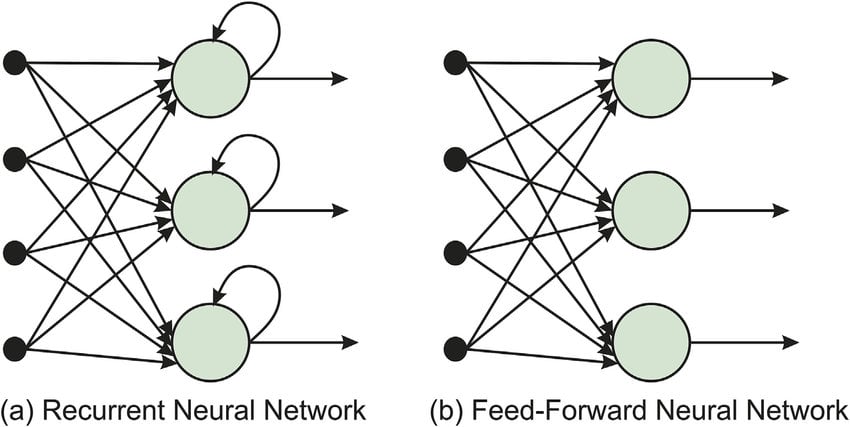
The key difference between these two architectures is that RNNs contain a continuous loop in the network that enables the input sequence to flow through the layers of the network many times. This characteristic enables RNNs to be very effective in processing sequential data, where an important part is to keep track of the ‘past’ of the sequence using some memory. The necessary memory block is represented by the hidden states that are used in the processing of the next inputs.

In the image below, we can see the two architectures that we compared where the ‘loop’ of the RNN is illustrated:

4. Types of RNNs

Throughout the years, many types of RNNs have been proposed to tackle the challenges that exist in RNNs. Now, let’s discuss the two most commonly used variations of RNNs.

4.1. LSTM

When an RNN processes very long sequences, the problem of vanishing gradients appears, meaning that the gradients of the loss function approach zero, making the network hard to train.

A Long Short-Term Memory Network (LSTM) is a variation of an RNN specifically designed to deal with the problem of vanishing gradients. It uses a memory cell that is able to maintain useful information for a long period of time without significantly decreasing the gradients of the network.

We can create an LSTM network using TensorFlow:

class LSTMModel(tf.keras.Model):
    def __init__(self, units, input_feature_dim, num_classes):
        super(LSTMModel, self).__init__()
        # LSTM layer
        self.lstm_layer = tf.keras.layers.LSTM(units, return_sequences=False, input_shape=(None, input_feature_dim))
        self.fc = tf.keras.layers.Dense(num_classes)
        
    def call(self, inputs):
        x = self.lstm_layer(inputs)
        output = self.fc(x)
        return output

And PyTorch:

import torch
import torch.nn as nn

class LSTMModel(nn.Module):
    def __init__(self, input_size, hidden_size, num_layers, num_classes):
        super(LSTMModel, self).__init__()
        self.hidden_size = hidden_size
        self.num_layers = num_layers
        # LSTM layer
        self.lstm = nn.LSTM(input_size, hidden_size, num_layers, batch_first=True)
        self.fc = nn.Linear(hidden_size, num_classes)
    
    def forward(self, x):
        # Initialize hidden state and cell state
        h0 = torch.zeros(self.num_layers, x.size(0), self.hidden_size).to(x.device)
        c0 = torch.zeros(self.num_layers, x.size(0), self.hidden_size).to(x.device)
        
        # Forward propagate LSTM
        out, _ = self.lstm(x, (h0, c0))  # out: tensor of shape (batch_size, seq_length, hidden_size)
        
        out = self.fc(out[:, -1, :])
        return out

4.2. GRU

Another common architecture is the Gated Recurrent Unit (GRU) which is similar to LSTMs but is much simpler in its structure and significantly faster when computing the output.

In TensorFlow, we can build a GRU network as follows:

import tensorflow as tf

class GRUModel(tf.keras.Model):
    def __init__(self, units, input_feature_dim, num_classes):
        super(GRUModel, self).__init__()
        # GRU layer
        self.gru_layer = tf.keras.layers.GRU(units, return_sequences=False, input_shape=(None, input_feature_dim))
        self.fc = tf.keras.layers.Dense(num_classes)
        
    def call(self, inputs):
        x = self.gru_layer(inputs)
        output = self.fc(x)
        return output

In PyTorch:

import torch
import torch.nn as nn

class GRUModel(nn.Module):
    def __init__(self, input_size, hidden_size, num_layers, num_classes):
        super(GRUModel, self).__init__()
        self.hidden_size = hidden_size
        self.num_layers = num_layers
        # GRU layer
        self.gru = nn.GRU(input_size, hidden_size, num_layers, batch_first=True)
        self.fc = nn.Linear(hidden_size, num_classes)
    
    def forward(self, x):
        h0 = torch.zeros(self.num_layers, x.size(0), self.hidden_size).to(x.device)
        
        # Forward propagate GRU
        out, _ = self.gru(x, h0)  # out: tensor of shape (batch_size, seq_length, hidden_size)
        
        out = self.fc(out[:, -1, :])
        return out

5. Applications

Now that we have gained an understanding of the architectures of RNNs, we’ll talk about their most common applications of them.

5.1. Natural Language Processing

The most common application of RNNs is in processing text sequences. For example, we can use an RNN to generate text by predicting each time the next word of a text sequence. This task can be proved helpful for chatbot applications and online language translators.

5.2. Series Forecasting

Another useful application of RNNs is in time series forecasting, where our goal is to predict some future outcomes given the previous ones. For example, in weather forecasting, we can use an RNN to explore historical patterns in previous weather data and employ them to predict the weather in the future better.

5.3. Video Processing

Videos can be considered as another type of sequence since they are sequences of image frames. So, RNNs can also be used in video processing tasks like video classification, where our goal is to classify a given video into a category.

5.4. Reinforcement Learning

Finally, RNNs are also used in cases where we want to make decisions in a dynamic environment, like in reinforcement learning. Specifically, we can control a robot using an RNN that maintains the current state of the environment in the RNN memory.

6. Conclusion

In this article, we presented RNNs. First, we talked about their architecture and their differences from traditional networks. Then, we briefly discussed two types of RNNs and some of their applications.