Introduction to Quantum Computing | Baeldung on Computer Science

1. Introduction

In this tutorial, we’ll understand the basics of quantum computing. Since this differs significantly from the classical computing we are all familiar with, we’ll also cover the basic principles. Then, we’ll go through the essential elements of quantum computing.

Further, the tutorial will also cover the current algorithms and infrastructure for practical quantum computing applications.

2. What Is Quantum Computing?

Quantum computing is a field of study centered on developing computer technology based on the principles of quantum theory. Quantum theory is an area of physics that explains how matter and energy behave at the atomic and subatomic levels.

2.1. Limitations of Classical Computing

Let’s first understand what we mean by classical computing. It’s basically binary computing, where we store information in bits. A bit is always in one of the two physical states, represented by a single binary value, usually a ‘0’ or a ‘1’.

Physically, bits are stored in memory through transistors laid out in a circuit. It’s able to hold charge by its internal capacitance. This charge determines the state of each bit, which, in turn, determines the bit’s value. Transistors are normally created using semiconductor material like Silicon:

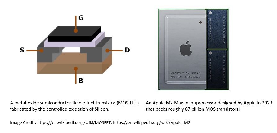
A microprocessor is an integrated circuitry (IC) responsible for processing instructions in classical computing. It generally comprises billions of transistors configured as thousands of individual digital circuits, each performing some specific logic function.

Over the last few decades, processors have got cheaper and more powerful, as reasonably predicted by Moore’s Law. However, there is a limit to the number of transistors we can pack in a digital circuit before hitting the restrictions of physical laws, especially at subatomic levels.

2.2. Advent of Quantum Computing

Quantum computing is based on the quantum mechanical phenomenon, which was introduced in the early twentieth century, long before classical computing became the mainstay. However, for decades quantum mechanics and computer science were distinct academic areas of study.

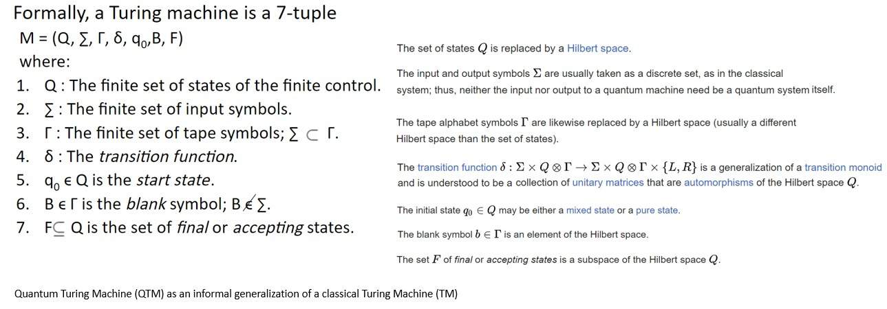
It was not until the late twentieth century, that these areas started to converge. In 1980, Paul Benioff introduced the idea of a Quantum Turing Machine (QTM) as a generalization of a Turing Machine (TM). It’s an abstract machine used to model the effects of a quantum computer:

Despite all the advancements, it wasn’t easy to simulate quantum dynamics with classical computers. Later, in the 1980s, Richard Feynman and Yuri Manin independently suggested that hardware based on quantum phenomena might be more efficient for such simulations.

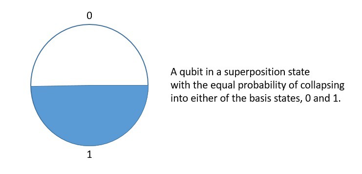
The basic unit of information in quantum computing is a qubit or quantum bit, similar to the bit in classical computing. However, unlike a bit, a qubit can exist in both its basis states simultaneously. In essence, a qubit is a two-state quantum-mechanical system!

3. Background of Quantum Mechanics

The evolution of quantum mechanics encompasses the work of scientists over more than two centuries. Classical mechanics described the natural world pretty well using the laws of motion and gravity. However, the scientific inquiry into the properties of light fell short of explanation based on the prevalent theories at that time.

3.1. Development of Old Quantum Theory

Issac Newton laid the foundation of the corpuscular theory of light. But the observed inconsistencies in experimentations led to the development of the wave theory of light. It was well described by the famous interference experiment by Thomas Young in 1803.

However, Gustav Kirchhoff described the black-body radiation problem in 1859 which challenged the wave theory of light. To describe black-body radiation, Max Plack postulated in 1900 that energy is radiated and absorbed in discrete “quanta”:

$E = h\nu ; \\ E = energy \hspace{2mm} of \hspace{2mm} a \hspace{2mm} photon \\ \nu = frequency \hspace{2mm} of \hspace{2mm} the \hspace{2mm} photon \\ h = Planck's \hspace{2mm} constant = 6.626 x 10^{-34} Joule.sec$

However, Planck never took his quantum hypothesis rather seriously. Although in 1905, Albert Einstein used Planck’s quantum hypothesis to explain the photoelectric effect, a name given to the emission of electrons when electromagnetic radiation hits a material.

Later, in 1924, Louis-Victor de Broglie hypothesized that all matter has a wave-like nature. It was soon proved experimentally for electrons with the observation of electron diffraction. Later, it was observed for larger particles like neutrons and protons:

$\lambda = \frac{h}{p}; \\ \lambda = de \hspace{2mm} Broglie \hspace{2mm} wavelength \hspace{2mm} associated \hspace{2mm} with \hspace{2mm} a \hspace{2mm} massive \hspace{2mm} particle \\ p = momentum \hspace{2mm} of \hspace{2mm} the \hspace{2mm} particle \\ h = Planck's \hspace{2mm} constant$

These and other contributions from scientists in the period from 1900 to 1925 are generally referred to as the “old quantum theory”. It’s basically a collection of heuristic corrections to classical mechanics rather than a complete theory of quantum mechanics.

3.1. Development of New Quantum Theory

After 1925, rigorous mathematical foundations were found to describe and unify different approaches in quantum theory. The groundbreaking works of Erwin Schrödinger, Werner Heisenberg, John von Neuman, Paul Dirac, and several others led to the “new quantum theory”.

A significant landmark in the development of quantum mechanics came when in 1926, Erwin Schrödinger came up with a linear partial differential equation governing the wave function of a quantum-mechanical system:

$i \hbar \frac{\partial}{\partial t}\left |\Psi(t)\right > = \hat H \left |\Psi(t)\right > ; \\ i = imaginary \hspace{2mm} unit \\ \hbar = reduced \hspace{2mm} Planck's \hspace{2mm} constant \\ t = duration \\ \left |\Psi(t)\right > = quantum \hspace{2mm} state \hspace{2mm} vector \\ \hat H = Hamiltonian \hspace{2mm} operator$

Another major milestone was when Werner Heisenberg postulated his uncertainty principle in 1927. It asserted a fundamental limit to the accuracy with which the values for certain pairs of physical quantities of a particle can be predicted from initial conditions:

$\Delta x \Delta p \geq \frac{h}{4\pi }; \\ \Delta x = uncertainty \hspace{2mm} in \hspace{2mm} position \\ \Delta p = uncertainty \hspace{2mm} of \hspace{2mm} momentum \\ h = Planck's \hspace{2mm} constant$

These and other scientific inquiries led toward the wave-particle duality, a notion that every quantum entity can be described as either a particle or a wave. While it explains a broad range of observed phenomena, it remains a subject of an ongoing conundrum in modern physics.

Starting around 1930, the ideas from the new quantum theory applied to electromagnetism gave rise to the Quantum Field Theory (QFT). It’s a theoretical framework combining classical field theory, special relativity, and quantum mechanics. It has led to several formulations like the Standard Model.

4. Fundamental Principles of Quantum Mechanics

A comprehensive description of a quantum-mechanical system is an advanced subject, much beyond the scope of this tutorial. However, the wave-particle duality of a quantum object leads to several interesting physical phenomena. This gives us several principles that form the foundation of quantum information science.

4.1. Quantum Superposition

Quantum superposition is one of the fundamental principles of quantum mechanics. It says a particle can be in a superposition of multiple quantum states or eigenstates. This contrasts classical mechanics, where things like position or momentum are always well-defined.

Mathematically, we can superimpose or add any two or more quantum states resulting in another valid quantum state. Conversely, we can represent a quantum state as a sum of two or more distinct states. It refers to the property of solutions to Schrödinger’s equation.

Interestingly, on interaction with the external world, the wave function reduces to a single eigenstate, called the wave function collapse. This connects the wave function with the classical observables like position and momentum. This is also the basis of measurements in quantum mechanics.

4.2. Quantum Entanglement

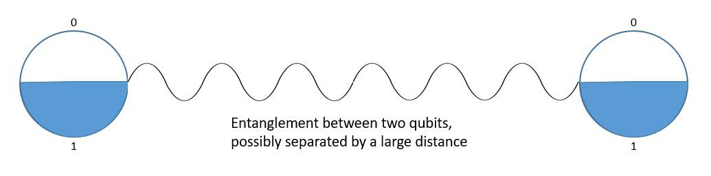
Quantum entanglement is the phenomenon that occurs when a group of particles is generated in a way such that the quantum state of each particle of the group can not be described independently of the state of the others, including when the particles are separated by a large distance.

As a result, measurement of physical properties such as position and momentum performed on entangled particles can, in some cases, be found to be perfectly correlated. This is of particular importance, as the mutual information between the entangled particles can be exploited.

Historically, entanglement has always been received with caution. For instance, the Einstein-Podolsky-Rosen paradox attempts to show that the quantum-mechanical description of physical reality given by wave function is incomplete. However, experiments have supported the existence of entanglement.

5. Elements of Quantum Computing

While quantum mechanics has come a long way in describing most of the natural world, gravity still remains out of reach, which is better explained by general relativity. Nonetheless, an interesting outcome of this quest has been the development of quantum information science, which combines the principles of quantum mechanics and information science.

5.1. Foundation of Qubit

A qubit is the basic unit of quantum information. Quantum information is the information on the state of a quantum system. Further, a qubit is a two-state quantum-mechanical system. This system can be a quantum particle like an electron or a photon.

The quantum property in the case of a photon is its polarization, and the two quantum states are vertical polarization and horizontal polarization. Similarly, the quantum property in the case of an electron is its spin, and the two quantum states are spin-up and spin-down:

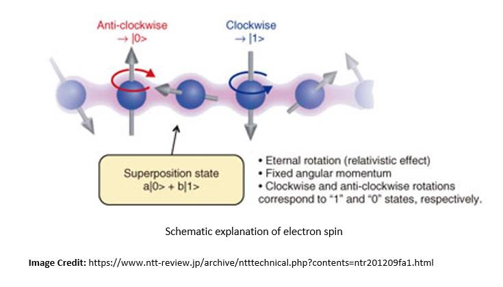
A qubit can exist in any quantum superposition of its two independent quantum states. Each possible quantum state has an associated probability amplitude. Upon measurement, the qubit’s state collapses to either of the two possible quantum states.

Quantum interference affects the state of a qubit to influence the probability of a certain outcome during measurement. While the properties of a single qubit are fascinating, the power of quantum computing comes from the use of multiple qubits:

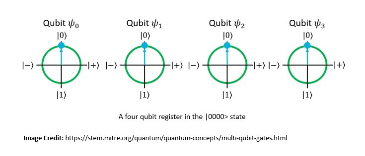
Quantum entanglement enables qubits separated by large distances to interact with each other instantaneously. This allows several qubits to act as a group and form a global system. It acts as a computational multiplier for qubits.

Consequently, the number of computations a quantum computer can undertake is $2^{n}$ where $n$ is the number of qubits used. The quantum properties of superposition and entanglement together create enormously enhanced computing power.

5.2. Representation of Qubit

Since a qubit can be in a superposition of its possible quantum states, its state is best described by a two-dimensional column vector. This is called the quantum state vector and has a unit norm, meaning the magnitude squared of its entries must sum to 1.

For instance, $\begin{bmatrix}\alpha \\ \beta\end{bmatrix}$ represents a valid qubit state if $\left| \alpha \right|^{2} + \left| \beta \right|^{2} = 1$ . Here $\alpha$ & $\beta$ can be any real or complex numbers.

The quantum state vectors $\begin{bmatrix}1 \\ 0\end{bmatrix}$ and $\begin{bmatrix}0 \\ 1\end{bmatrix}$ form the basis vectors and functionally correspond to the two states of a classical bit. We can represent any quantum state vector as the sum of the basis vectors:

$\begin{bmatrix}x \\ y\end{bmatrix} = x \begin{bmatrix}1 \\ 0\end{bmatrix} + y \begin{bmatrix}0 \\ 1\end{bmatrix}$

Now, when we measure the quantum state vector $\begin{bmatrix}\alpha \\ \beta\end{bmatrix}$ , its yields the outcome as 0 with probability $\alpha ^{2}$ and the outcome as 1 with probability $\beta^{2}$ . Consequently, the qubit’s new state becomes $\begin{bmatrix}1 \\ 0\end{bmatrix}$ or $\begin{bmatrix}0 \\ 1\end{bmatrix}$ respectively.

5.3. Alternate Representations

While row and column vector notation is generally used in linear algebra, it’s unsuitable for quantum computing. This is especially true when dealing with multiple qubits. It leads to ambiguity about the space of vectors and makes expressing even simple vectors quite cumbersome.

Hence, in quantum mechanics, Dirac notation is ubiquitously used to denote quantum states. It was developed by Paul Dirac as the bra-ket notation. The notation uses angle brackets ‘<‘ and vertical bars ‘|’ to construct “bras” and “kets”. We can represent the single-qubit basis states in Dirac’s notations as:

$\begin{bmatrix}1 \\ 0\end{bmatrix} = \left| 0 \right> , \begin{bmatrix}0 \\ 1\end{bmatrix} = \left| 1 \right>$

For instance, if $\phi$ is a row vector, we can represent it as a bra-vector $\left<\phi \right|$ . Similarly, if $\psi$ is a column vector, we can represent it as a ket-vector $\left|\psi \right>$ . Hence, if $\phi$ & $\psi$ are quantum state vectors, $\left<\phi|\psi\right>$ represents their inner product.

Physicist Felix Bloch developed the Bloch sphere, a geometrical representation of the pure state space of a two-level quantum mechanical system. It’s basically a unit 2-sphere with antipodal points corresponding to the orthogonal state vectors:

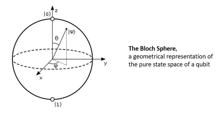
The north and south poles of the Bloch sphere are typically chosen to correspond to the standard basis vectors $\left| 0 \right>$ & $\left| 1 \right>$ respectively. The points on the surface of the sphere correspond to the pure states of the system, and the interior points correspond to the mixed states.

5.4. Quantum Operations & Linear Algebra

Linear algebra is the language of quantum computing and forms the basis for its mathematical representation. It’s widely used to describe qubit states and quantum operations and predict what a quantum computer does in response to a sequence of instructions.

We’ve seen how to represent the state of a single qubit using vectors. Now, the state of two qubits can be represented using the tensor product of their individual quantum state vectors:

$\begin{bmatrix}a \\ b \end{bmatrix} \otimes \begin{bmatrix}c \\ d \end{bmatrix} = \begin{bmatrix}a \begin{bmatrix}c \\ d \end{bmatrix} \\ b \begin{bmatrix}c \\ d \end{bmatrix} \end{bmatrix} = \begin{bmatrix}ac \\ ad \\ bc \\ bd\end{bmatrix}$

We can also represent quantum operations using a matrix. When a quantum operation is applied to a qubit, we can multiply the two matrices and get the new state of the qubit after the operation:

$H = \frac{1}{\sqrt{2}}\begin{bmatrix}1 & 1 \\ 1 & -1 \end{bmatrix} \newline H \begin{bmatrix}a \\ b \end{bmatrix} = \frac{1}{\sqrt{2}}\begin{bmatrix}1 & 1 \\ 1 & -1 \end{bmatrix} \begin{bmatrix}a \\ b \end{bmatrix} = \frac{1}{\sqrt{2}}\begin{bmatrix}1 \\ 1 \end{bmatrix}$

Here, we are using the Hadamard transformation ( $H$ ) to put a qubit( $\begin{bmatrix}1 \\ 0 \end{bmatrix}$ ) in a superposition state where it has an even probability of collapsing to either ‘0’ or ‘1’.

Further, quantum mechanics is mathematically formulated in the Hilbert space, which allows generalizing the methods of linear algebra and calculus from finite-dimensional Euclidean vector spaces to spaces that may be infinite-dimensional.

In quantum mechanics, a quantum state is typically represented as an element of a complex Hilbert space, for example, the infinite-dimensional vector space of all possible wave functions or some more abstract Hilbert space constructed more algebraically.

5.5. Quantum Gates & Circuits

There are multiple approaches to building quantum computers from the basic unit of qubits. One of the models is quantum circuits, in which a computation is a sequence of quantum gates, measurements, initialization of qubits to known values, and possibly other actions.

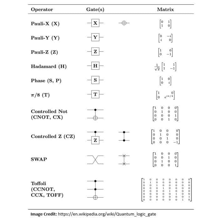
A quantum logic gate is a basic quantum circuit operating on a small number of qubits. It’s functionally equivalent to classical logic gates in conventional digital circuits. However, unlike classical logic gates, quantum logic gates are reversible:

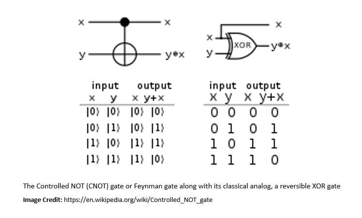
Quantum gates are unitary operators and are described as unitary matrices relative to some basis, usually the computational basis. The current notation of quantum gates has been built on top of the notation introduced by Richard Feynman in 1986.

For instance, a simple quantum logic gate is the Identity gate which we can define for a single qubit as:

$I = \begin{bmatrix}1 & 0 \\ 0 & 1\end{bmatrix}$

Here, $I$ is basis independent and does not modify the quantum state. Several other quantum gates have been defined by various authors:

The minimum set of actions that a quantum circuit needs to be able to perform on the qubits to enable quantum computation is known as DiVincenzo’s criteria. It was proposed in 2000 by David P. DiVincenzo as seven conditions an experiment must satisfy to implement quantum algorithms.

The graphical depiction of quantum circuit elements is described using a variant of the Penrose graphical notation, a visual depiction of tensors proposed by Roger Penrose in 1971. A quantum circuit that performs teleportation of a qubit is depicted below:

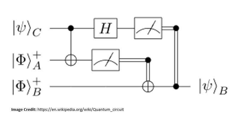
In a quantum circuit, time flows from left to right, and hence, the gates are ordered chronologically. Here, the quantum logic gate depicted by ‘H’ is a Hadamard operation acting on a single-qubit register. The other operation in this circuit is a measurement denoted by the meter symbol.

6. Quantum Algorithms

A Quantum algorithm, like a classical algorithm, is a step-by-step procedure for solving a problem. However, in the case of a quantum algorithm, each step can be performed on a quantum computer. These run on a realistic model of quantum computation, like the quantum circuit model of computation. Further, they may use some features of quantum computing, like superposition and entanglement.

To study the hardness of computational problems addressed by quantum algorithms, we need new complexity classes. Quantum complexity theory deals with the complexity classes defined using quantum computers. Two important quantum complexity classes are Bounded-error Quantum Polynomial-time (BQP) and Quantum Merlin Arthur (QMA), analogous to classical complexity classes, P and NP.

6.1. Quantum Fourier Transform

The Quantum Fourier Transform (QFT) is a linear transformation on quantum bits and is the quantum analogue of the Discrete Fourier Transform (DFT). In mathematics, a Fourier transform is a transform that converts a function into a form that describes the frequencies present in the original function:

Introduced by Joseph Fourier, the Fourier Transform (FT) is a fundamental tool of classical analysis and is just as important for quantum computation. In fact, the efficiency of QFT far surpasses what is possible on a classical machine. Hence, QFT is a part of many quantum algorithms.

For instance, Shor’s algorithm for finding the prime factors of an integer. Developed in 1994 by Peter Shor, Shor’s algorithm runs in polylogarithmic time. The efficiency of Shor’s algorithm is due to the efficiency of the QFT and modular exponentiation by repeated squaring:

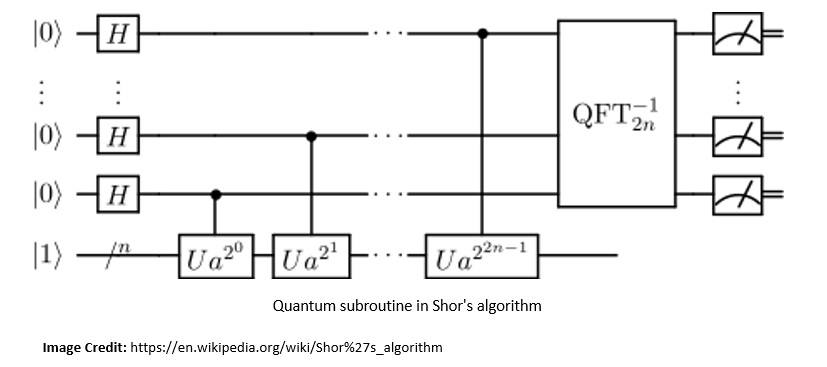
With a quantum computer with a sufficient number of qubits, it’s theoretically possible to break public-key cryptographic systems like the RSA scheme. This led to the research into new cryptosystems that are secure from quantum computers, collectively known as post-quantum cryptography.

6.2. Amplitude Amplification

Amplitude amplification is another very important tool in quantum computing on which many quantum algorithms are based. It was discovered by Gilles Brassard and Peter Høyer and later independently by Lov Kumar Grover. It can be used to obtain a quadratic speedup over several classical algorithms.

The central idea behind amplitude amplification is to amplify the probability of the desired outcome occurring by performing a sequence of reflections. These reflections rotate the initial state closer toward a desired target state.

Amplitude amplification comes from the idea behind Grover’s algorithm, proposed by Lov Grover in 1996. It’s also known as the quantum search algorithm and is regarded as the second major algorithm proposed for quantum computing:

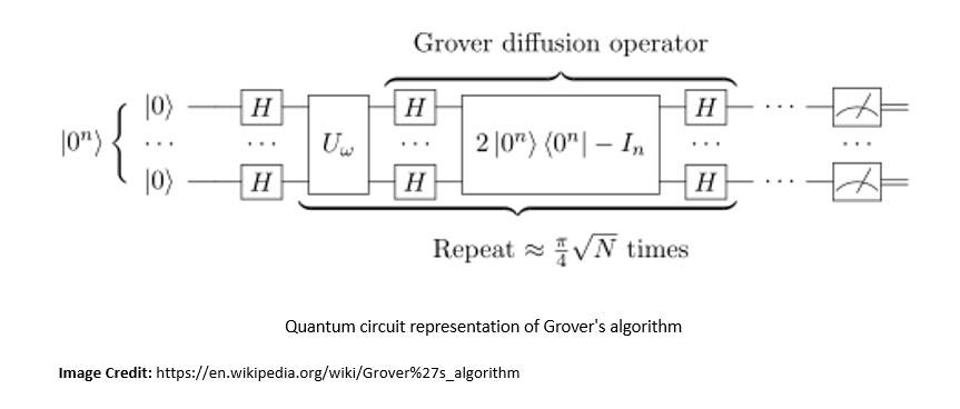
Grover’s algorithm is a quantum algorithm for unstructured search that finds with high probability the unique input to a black box function that produces a particular output value. This and other amplitude amplification algorithms can be used to speed up a broad range of algorithms.

7. Quantum Infrastructure

While the field of quantum computing is decades old now, a practical quantum computer is still in its infancy. There is immense potential in terms of applications of quantum computing. Hence, large companies have been investing significantly in hardware research. However, there are still significant challenges in delivering scalable quantum computing infrastructure for solving real-world problems.

7.1. Approaches for Quantum Computing

There are two primary theoretical approaches for quantum computing; analog and digital gate-based quantum computing. The motivation is to finally achieve a universal quantum computer employing thousands of qubits and capable of solving a broad class of problems.

Analog quantum computing includes approaches like quantum annealing, quantum simulation, and adiabatic quantum computing:

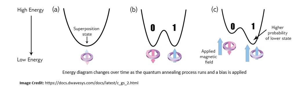
Analog quantum computers are relatively easier to achieve but have limited advantages over classical computing and hence specific applications.

Gate-based quantum computing is more universal in nature and uses quantum circuits composed of qubits whose state is manipulated through quantum gates. A class of gate-based quantum computers is known as Noisy Intermediate-Scale Quantum (NISQ), which operates without full error correction.

7.2. Challenges in Quantum Computing

The power of quantum computing comes from the ability to precisely control coherent quantum systems, a superposition of multiple entangled qubits. However, quantum systems that are not perfectly isolated are prone to decoherence caused by several environmental factors like electromagnetic waves.

Decoherence is the loss of quantum coherence and hence the loss of information from a system into the environment:

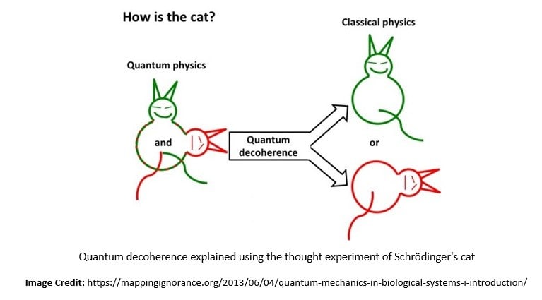
For quantum computations to take place, we require the coherence of states to be preserved and decoherence to be managed. This is a big challenge in constructing quantum computers.

Quantum error correction strives to achieve fault-tolerant quantum computing by reducing the effects of decoherence and other quantum noise. There can be several ways for error correction, for instance, spreading the information of one qubit onto a highly entangled state of several qubits.

7.3. Physical Realization of Qubit

The area of practical quantum computers is in its early infancy. This is evident from the number of candidates that have been proposed and actively researched for the physical realization of a qubit. Of course, it’s a very difficult task due to the inherent challenges.

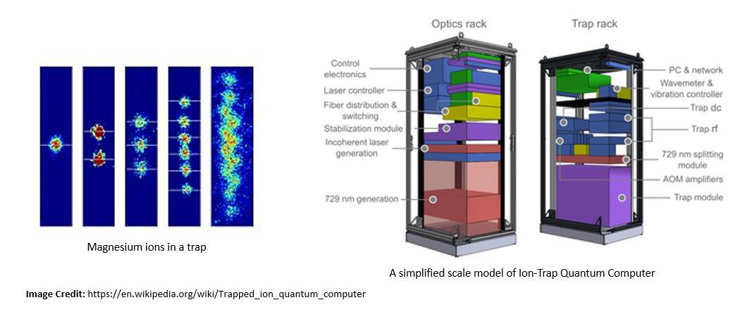
One of the popular approaches for constructing large-scale quantum computers is the trapped ion quantum computer. Here, ions are confined and suspended in a free space using electromagnetic fields, and qubits are stored in stable electronic states of each ion:

Another significant approach is superconducting quantum computing. It uses superconducting qubits as artificial atoms. For superconducting qubits, the two logic states are the ground state and the excited state. Several companies are investing in the research of superconducting quantum computing.

7.4. Applications of Quantum Computing

It’s important to understand that quantum computing is not a replacement for classical computing. Quantum computing is suitable for solving the class of problems which is almost out of reach for classical computing. For instance, difficult combinatorics problems in graph theory and statistics.

In any case, classical and quantum computers will have to work in tandem. In most practical applications, the architecture of the quantum computer will consist of classical and quantum parts:

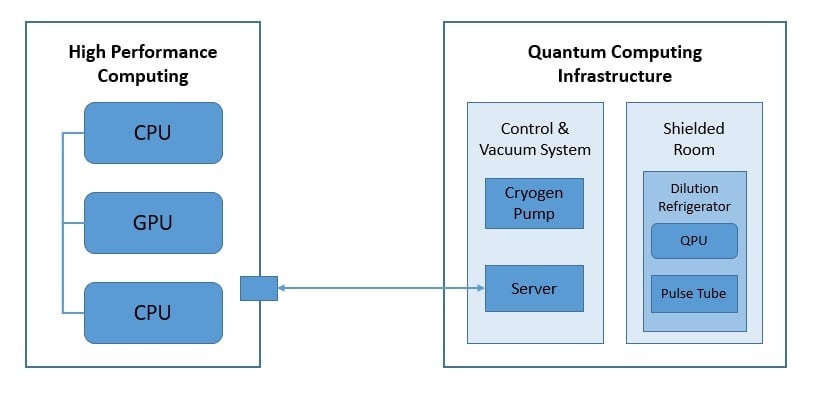
The architecture here presents a hybrid classical-quantum computer where applications interface with Quantum Processing Units (QPU) and their classical counterparts, CPUs, and GPUs.

There are several areas where quantum computing can make a sizable impact soon. For instance, quantum machine learning; integration of quantum algorithms within machine learning programs. It significantly improves the computational speed and data storage for machine learning.

7.5. Quantum Supremacy & Quantum Cloud Computing

Quantum supremacy is the goal of demonstrating that a programmable quantum device can solve a problem that no classical computer can solve in any feasible amount of time. Interestingly, the problem here does not have to be useful!

The term was coined by John Preskill in 2012. Notably, Google announced in 2019 that it had achieved quantum supremacy with the Sycamore processor, an array of 54 qubits:

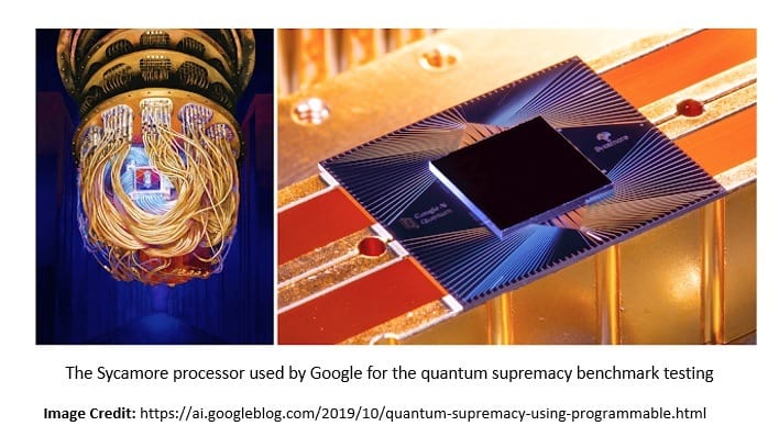
It was used to perform a series of operations in 200 seconds that would take a supercomputer about 10,000 years to complete!

Many companies have started to offer tools for quantum computing and cloud access to their quantum emulators, simulators, or processors. For instance, IBM Quantum by IBM, Azure Quantum by Microsoft, Quantum AI by Google, and Amazon Braket by Amazon.

8. Conclusion

In this tutorial, we covered the basic principles of quantum computing built on top of quantum mechanics. This included the core principles of quantum mechanics, like superposition and entanglement, and the basic elements of quantum computing, like qubits. Further, we covered a few quantum algorithms and a brief discussion of the current state of quantum infrastructure.

The idea of quantum computing is deeply rooted in quantum mechanics, which can be overwhelming to those without sufficient background in physics. Moreover, its mathematical formulation requires a good understanding of linear algebra and calculus. Even though it’s not necessary to master them to work with quantum computers, it certainly makes the journey easier.

Full Archive

About Baeldung

Core Concepts

Operating Systems

Artificial Intelligence

Graph Theory

Latex