Polynomial Addition and Multiplication Using Linked List

1. Introduction

In mathematics, a polynomial is an expression that contains a sum of powers in one or more variables multiplied by coefficients. A polynomial in one variable, $x$ , with constant coefficients is like: $a_0+a_1x+a_2x^2+...+a_{n-1}x^{n-1}+a_nx^n$ . We call each item, e.g., $a_nx^n$ , a term. If two terms have the same power, we call them like terms.

In this tutorial, we’ll show how to add and multiply two polynomials using a linked list data structure.

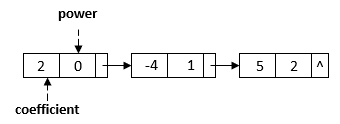
2. Represent a Polynomial with a Linked List

We can use a linked list to represent a polynomial. In the linked list, each node has two data fields: coefficient and power. Therefore, each node represents a term of a polynomial. For example, we can represent the polynomial $2-4x+5x^2$ with a linked list:

We can sort a linked list in $O(n\log n)$ time, where $n$ is the total number of the linked list nodes. In this tutorial, we’ll assume the linked list is ordered by the power for the simplicity of our algorithms.

3. Add Two Polynomials

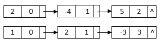
To add two polynomials, we can add the coefficients of like terms and generate a new linked list for the resulting polynomial. For example, we can use two liked lists to represent polynomials $2-4x+5x^2$ and $1+2x - 3x^3$ :

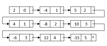
When we add them together, we can group the like terms and generate the result $3 - 2x^2 + 5x^2 - 3x^3$ :

Since both linked list are ordered by the power, we can use a two-pointer method to merge the two sorted linked list:

algorithm PolynomialAdd(head1, head2):
    // INPUT
    //    head1 = Head pointer of the first polynomial linked list
    //    head2 = Head pointer of the second polynomial linked list
    // OUTPUT
    //    Head pointer of the new polynomial linked list representing the sum
    head <- tail <- null
    p1 <- head1
    p2 <- head2
    while p1 != null and p2 != null: 
        if p1.power > p2.power:
            tail <- append(tail, p1.power, p1.coefficient)
            p1 <- p1.next
        else if p2.power > p1.power:
            tail <- append(tail, p2.power, p2.coefficient)
            p2 <- p2.next
        else:
            coefficient <- p1.coefficient + p2.coefficient
            if coefficient != 0:
                tail <- append(tail, p1.power, coefficient)
            p1 <- p1.next
            p2 <- p2.next
        if head is null:
            head <- tail
    while p1 != null:
        tail <- append(tail, p1.power, p1.coefficient)
        p1 <- p1.next
    while p2 != null:
        tail <- append(tail, p2.power, p2.coefficient)
        p2 <- p2.next
    return head

In this algorithm, we first create two pointers, $p1$ and $p2$ , to the head pointers of the two input polynomials. Then, we generate the new polynomial nodes based on the powers of these two pointers. There are three cases:

$p1$ ‘s power is greater than $p2$ ‘s power: In this case, we append a new node with $p1$ ‘s power and coefficient. Also, we move $p1$ to the next node.
$p2$ ‘s power is greater than $p1$ ‘s power: In this case, we append a new node with $p2$ ‘s power and coefficient. Also, we move $p2$ to the next node.
$p1$ and $p2$ have the same power: In this case, the new coefficient is the total of $p1$ ‘s coefficient and $p2$ ‘s coefficient. If the new coefficient is not $0$ , we append a new node with the same power and the new coefficient. Also, we move both $p1$ and $p2$ to the next nodes.

After that, we continue to append the remaining nodes from $p1$ or $p2$ until we finish the calculation on all nodes.

The $append$ function can create a new linked list node based on the input $power$ and $coefficient$ . Also, it appends the new node to the $tail$ node and returns the new $tail$ node:

algorithm Append(tail, power, coefficient):
    // INPUT
    //    tail = The last node of the current polynomial linked list
    //    power = The power of the new term to append
    //    coefficient = The coefficient of the new term to append
    // OUTPUT
    //    The new tail node after appending the new term
    new_node <- create a new node with power and coefficient
    if tail != null:
        tail.next <- new_node
    return new node

This algorithm traverses each linked list node only once. Therefore, the overall running time is $O(n + m)$ , where $n$ and $m$ are the number of terms for the two input polynomials.

4. Multiply Two Polynomials

To multiply two polynomials, we can first multiply each term of one polynomial to the other polynomial. Suppose the two polynomials have $n$ and $m$ terms. This process will create a polynomial with $n\times m$ terms.

For example, after we multiply $2-4x+5x^2$ and $1+2x - 3x^3$ , we can get a linked list:

This linked list contains all terms we need to generate the final result. However, it is not sorted by the powers. Also, it contains duplicate nodes with like terms. To generate the final linked list, we can first merge sort the linked list based on each node’s power:

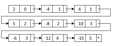
After the sorting, the like term nodes are grouped together. Then, we can merge each group of like terms and get the final multiplication result:

We can describe these steps with an algorithm:

algorithm PolynomialMultiply(head1, head2):
    // INPUT
    //    head1 = Head pointer of the first polynomial linked list
    //    head2 = Head pointer of the second polynomial linked list
    // OUTPUT
    //    Head pointer of the new polynomial linked list representing the product
    head <- null
    tail <- null
    p1 <- head1
    while p1 != null:
        p2 <- head2
        while p2 != null:
            power <- p1.power + p2.power
            coefficient <- p1.coefficient * p2.coefficient
            tail <- append(tail, power, coefficient)
            if head is null:
                head <- tail
            p2 <- p2.next
        p1 <- p1.next
    head <- mergesort(head)
    mergeLikeTerms(head)
    return head

In this algorithm, we first use a nested $while$ loop to multiply all term pairs from the two polynomials. This takes $O(nm)$ time, where $n$ and $m$ are the number of terms for the two input polynomials. Also, this process creates a linked list with $n\times m$ nodes.

Then, we merge sort the linked list based on each node’s power. This process takes $O(nm\log (nm))$ time.

After we sort the linked list, we can use a two-pointer approach to merge the like terms:

algorithm MergeLikeTerms(head):
    // INPUT
    //    head = Head pointer of the polynomial linked list
    // OUTPUT
    //    Modify the linked list in place by merging like terms
    prev <- null
    p1 <- head
    while p1 != null:
        p2 <- p1.next
        while p2 != null and p2.power = p1.power:
            p1.coefficient <- p1.coefficient + p2.coefficient
            p2 <- p2.next
            p1.next <- p2
        if p1.coefficient = 0 and prev != null:
            prev.next <- p2
        else:
            prev <- p1
        p1 <- p2

In this approach, we use one pointer as the start of a like term group and use another pointer to traverse the like terms in the same group. Each time we find a like term, we add its coefficient to the start like term node. Once we finish one like term group, we move the start pointer to the next group and repeat the same process to merge like terms. The running time of this process is $O(nm)$ as we need to visit $n\times m$ nodes.

Overall, the running time is $O(nm) + O(nm\log (nm)) + O(nm) = O(nm\log (nm) )$ .

5. Conclusion

In this tutorial, we showed how to represent a polynomial with the linked list data structure. Also, we showed two algorithms to add and multiply two linked list representations of polynomials.

Core Concepts

Operating Systems

Neural Networks

Graph Theory

Latex

Full Archive

About Baeldung

1. Introduction

2. Represent a Polynomial with a Linked List

3. Add Two Polynomials

4. Multiply Two Polynomials

5. Conclusion