

Learn through the super-clean Baeldung Pro experience:
>> Membership and Baeldung Pro.
No ads, dark-mode and 6 months free of IntelliJ Idea Ultimate to start with.
Last updated: February 28, 2025
Learn through the super-clean Baeldung Pro experience:
>> Membership and Baeldung Pro.
No ads, dark-mode and 6 months free of IntelliJ Idea Ultimate to start with.
One Class Support Vector Machines (SVMs) are a type of outlier detection method.
In this tutorial, we’ll explore how SVMs perform outlier detection and illustrate its utility with a simple example.
Let’s start with the basics.
Usually, SVMs aim to generalize from some input data. With this, they can decide whether any additional data are outliers or not.
Basic SVMs do this by separating data into several classes. From there, they can decide which class any subsequent data belongs to.
One Class SVMs are similar, but there is only one class. Therefore, a boundary is decided on using the available data. Any new data that lies outside that boundary is classed as an outlier.
To see how this is done, let’s dive into the formulation.
There are two formulations of One Class SVMs. The first is by Schölkopf, which involves using a hyperplane (a plane in n-dimensions) for the decision boundary. The second is by Tax and Duin, which uses a hypersphere for the decision boundary. Let’s explore the latter.
The hypersphere is characterized by a center  with a radius
  . Also, let’s say we have
  data points that are given by
  , where
  .
.
Therefore, the Euclidean distance from the hypersphere center and a given data point is  . We want to minimize a cost function
  with the constraint that every point lies within or on the hypersphere. Therefore, our constraint is
  .
.
As it stands, outliers will greatly affect the tuning. Let’s address this by modifying the cost function to  and the constraint to
  .
.
 are the positive weights associated with each data point. The higher it is, the less that particular data point affects the tuning of
  . Also,
  provides a trade-off between volume and classification errors.
Combining this with the method of Lagrange Multipliers, we are left with an optimization problem to solve:
(1) 
where  and
and  are non-negative Lagrange multipliers.
  should be maximized with respect to and , but minimized with respect to
  and .
and .
Now let’s apply this to a simple problem!
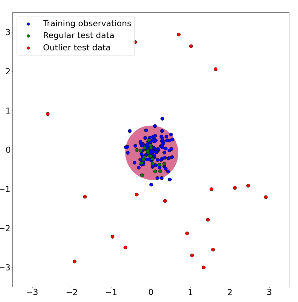
Suppose we train a One Class SVM on 100 data points from a two-dimensional Gaussian distribution  .
.
After that, we add both 20 additional data points and 20 data points drawn from a Uniform distribution  . Our goal is to correctly classify the Gaussian data points while ignoring the outlier data from the Uniform distribution.
This is the result:
In this brief article, we showed how they differ from basic SVMs. Then, we outlined the relevant equations and applied them to a simple example.