

Learn through the super-clean Baeldung Pro experience:
>> Membership and Baeldung Pro.
No ads, dark-mode and 6 months free of IntelliJ Idea Ultimate to start with.
Learn through the super-clean Baeldung Pro experience:
>> Membership and Baeldung Pro.
No ads, dark-mode and 6 months free of IntelliJ Idea Ultimate to start with.
Some algorithms base their ideas on the binary representation of integer numbers. In this tutorial, we’ll demonstrate two algorithms to finding the most significant bit in an integer number.
We’ll start by providing some definitions that should help us understand the provided approaches. After that, we’ll explain the naive approach and use some facts to get a better approach with lower time complexity.
Let’s introduce a quick reminder of transforming a non-negative integer number from the decimal into the binary format. After that, we’ll introduce the bitwise operations and an equation that we’ll need later to optimize the naive approach.
Let’s provide an example to explain the idea. Suppose the number is 89, and we want to represent it using the binary format.
Take a look at the steps to do this:
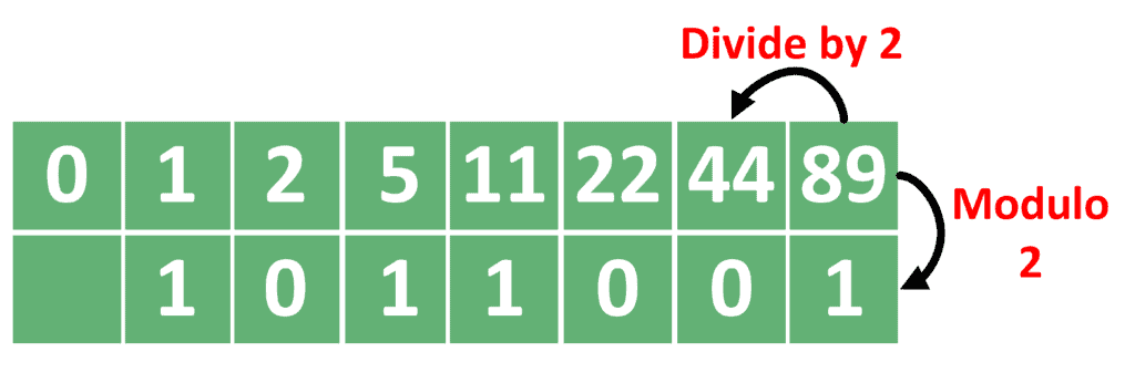
We perform multiple steps until the number reaches zero. In each step, we divide the number by 2. Also, we get the modulo of the number after dividing it by two and add it to the answer.
In the end, the answer is the list of zeros and ones we got when taking the modulo of the number when divided by 2.
Note that the most significant bit is the last one we store. Similarly, the least significant bit is the first one we get.
Most programming languages support bitwise operations to be applied to non-negative integers. The use of these operations is to manipulate the bits of the binary representation of a certain number.
For this article, we’re interested in the left shifting operation denoted as  . This operation shifts the binary format of a number by a specific amount of bits to the left. For example,
  means shifting the bit 1 by
  times to the left. The resulting number is
  , because it only has the
  bit activated, while all the other ones are turned off.
The interesting thing about binary numbers is the following equation:
![\[\boldsymbol{\sum_{i=0}^{k}2^{i} = 2^{k+1} - 1}\]](/wp-content/ql-cache/quicklatex.com-953295fca69c7105adcf91e34a1b43bb_l3.svg "Rendered by QuickLaTeX.com")
From this equation, we can conclude that:
![\[\boldsymbol{\sum_{i=0}^{k}2^{i} < 2^{k+1}}\]](/wp-content/ql-cache/quicklatex.com-54d7fd84fd2471aa279fde78486b9842_l3.svg "Rendered by QuickLaTeX.com")
What this means is that each bit  when activated, has a larger value than the sum of all the smaller bits, even if all of them are activated as well. This observation will help us when we improve the naive approach later.
For the naive approach, we’ll extract the bits of the binary representation one by one. For each bit, we check its value and store the most significant active one.
Take a look at the implementation of the naive approach:
algorithm NaiveMSB(n):
    // INPUT
    //     n = the non-negative number
    // OUTPUT
    //     Returns the index of the most significant bit (msb)

    index <- 0
    msb <- -1

    while n > 0:
        bit <- n mod 2
        n <- n / 2
        if bit = 1:
            msb <- index
        index <- index + 1

    return msb
We start by initializing the  with zero that indicates the current bit index. We also set
  to be -1, which will store the index of the most significant bit.
After that, we perform multiple steps. In each step, we get the value of the current bit by taking the remainder after dividing  by 2. Also, we divide by 2 to move to the next step. Note that these steps are similar to getting the binary representation of the number we explained in section 2.1.
For each bit, we check whether it’s activated or not. If so, we store its index as the most significant bit found so far. Also, we increase the by one to move to the next bit.
Once reaches zero, it means we’ve iterated over all the bits of . At this point, we return the required index.
It’s worth noting that in the case when was zero, then the  loop won’t be executed. The algorithm returns -1, indicating that doesn’t have any activated bits.
The complexity of the naive approach is  , where is the required non-negative number.
First of all, let’s explain the idea behind using the binary search algorithm to solve this problem. Then, we can implement the algorithm.
In section 2.3, we noticed that the value of each bit is larger than the value of all the lower bits, even if all of them are activated. We can use this fact to find the next bit to the most significant one. By the next bit, we mean the bit  , where is the most significant one.
Rather than performing a linear search to find this bit, we can use the binary search algorithm.
In the beginning, we need to know the maximum index that could be the answer. Let’s denote this value as  . The answer is located somewhere inside the range
 ![[0, MAX]](/wp-content/ql-cache/quicklatex.com-9a954c21301a0388d25be23fd09a9282_l3.svg "Rendered by QuickLaTeX.com") .
.
To find the bit next to the most significant one, we check the middle of the searching range. Let’s assume the current searching range is ![[L, R]](/wp-content/ql-cache/quicklatex.com-aeea634230c22e2940acb7070696d9ef_l3.svg "Rendered by QuickLaTeX.com") , and the middle value is
, and the middle value is  .
.
If  is larger than
  , then this could be the needed bit. In this case, we can conclude that the bit is either this one or a smaller one. Thus, it’s somewhere inside the range
 ![\boldsymbol{[L, mid - 1]}](/wp-content/ql-cache/quicklatex.com-5d2c3cc4ec1c015c7d87c09e921cd85f_l3.svg "Rendered by QuickLaTeX.com") .
.
However, if is not larger than , then this bit can’t be the next one to the most significant. Therefore, the searching range becomes ![\boldsymbol{[mid + 1, R]}](/wp-content/ql-cache/quicklatex.com-91064e3183f046d1c3ab7bd756394661_l3.svg "Rendered by QuickLaTeX.com") because we need to try and increase the index of the bit.
because we need to try and increase the index of the bit.
Let’s use these ideas to implement the binary search approach.
Take a look at the implementation of the binary search approach:
algorithm BinarySearchMSB(n):
    // INPUT
    //     n = the non-negative number
    // OUTPUT
    //     Returns the index of the most significant bit (msb)

    msb <- -1
    L <- 0
    R <- MAX + 1
    while L <= R:
        mid <- (L + R) / 2
        if (1 << mid) > n:
            msb <- mid - 1
            R <- mid - 1
        else:
            L <- mid + 1

    return msb
First of all, we initialize  and
and  as the searching range. As we can see, starts from zero, while starts from the maximum possible answer . We added one to because we’re searching for the next bit to the most significant one.
Also, we initialize that will hold the index of the most significant bit.
In each step of the binary search operation, we calculate the middle point of the searching range. Then, we check whether the bit has a larger value than . If so, then we have a possible answer.
In this case, we store the bit before this one as a possible answer so far. We also move the right side of the searching range  to be
to be  because we should try to check smaller values.
On the other hand, if the value of the  bit isn’t larger than , then we move the left side of the searching range
  to be
to be  . This is because we need to search for larger values.
In the end, we return the stored answer .
The complexity of the naive approach is  , where is the required number. The reason is that we’re performing a binary search operation over the bits of . Since the number of bits of is
  , and we’re performing a binary search operation, then the complexity will be the logarithmic value of the number of bits.
Let’s take the same example described in section 2.1 and see how can both algorithms calculate the most significant bit. In that example, was equal to 89.
Check the table that describes the steps of the algorithm:
| index | n | bit | msb |
|---|---|---|---|
| 0 | 89 | 1 | 0 |
| 1 | 44 | 0 | 0 |
| 2 | 22 | 0 | 0 |
| 3 | 11 | 1 | 3 |
| 4 | 5 | 1 | 4 |
| 5 | 2 | 0 | 4 |
| 6 | 1 | 1 | 6 |
| 0 |
Mainly, we’re extracting the bits of one by one. In each step, if the  equals to one, we store the current as the .
In the end, we’ll have the resulting .
For the binary search, we’ll use a similar  , but we’ll assume that equals 8. Let’s see how well the algorithm work:
|
|
|
|

|
|
|---|---|---|---|---|
| 0 | 9 | 4 | 16 | -1 |
| 5 | 9 | 7 | 128 | 6 |
| 5 | 6 | 5 | 32 | 6 |
| 6 | 6 | 6 | 64 | 6 |
| 7 | 6 |
In each step, we calculate the middle point of the range . Then, we compare  with and decide whether to look for the answer in the left or the right side of the range. Also, when is larger than , we store
  as the current .
As we can see, in the binary search approach, we ended up making a lower number of comparisons.
As we can see, using the binary search operation gives us a lower complexity. However, there’s one primary condition to be able to use the binary search operation. We must have an upper bound for the possible answer to initialize with .
If we can’t estimate the upper bound for the most significant bit index, then we should go with the naive approach whose complexity isn’t that bad.
In this tutorial, we discussed the problem of finding the most significant bit for a given non-negative integer.
We presented a few ideas related to the binary representation of a given non-negative integer. Based on these ideas, we were able to develop a naive approach and optimize it to reach the binary search approach.
In the end, we presented a quick comparison between both of them and showed the requirements for using the binary search approach.