Determining the Most Distant Pair of Points | Baeldung on Computer Science

1. Overview

In this tutorial, we’ll talk about the problem of finding the distance between the farthest pair of points from a given set of points.

First, we’ll define the problem and provide an example to explain it. Then, we’ll present two different approaches to solving it and work through their implementations and time complexity.

2. Defining the Problem

Suppose we have a set of $N$ points in a cartesian coordinate on the $2D$ plane. We were asked to find the maximum distance between all the possible pairs of points. (Recall the distance between two points $\boldsymbol{P}$ and $\boldsymbol{Q}$ equals the Euclidean distance $\boldsymbol{\sqrt{(P.x - Q.x)^{2} + (P.y - Q.y)^{2} } }$ ).

Let’s take a look at the following example:

Given an $N = 3$ and points $P_1(0, 3)$ , $P_2(0, 0)$ and $P_3(4, 0)$ :

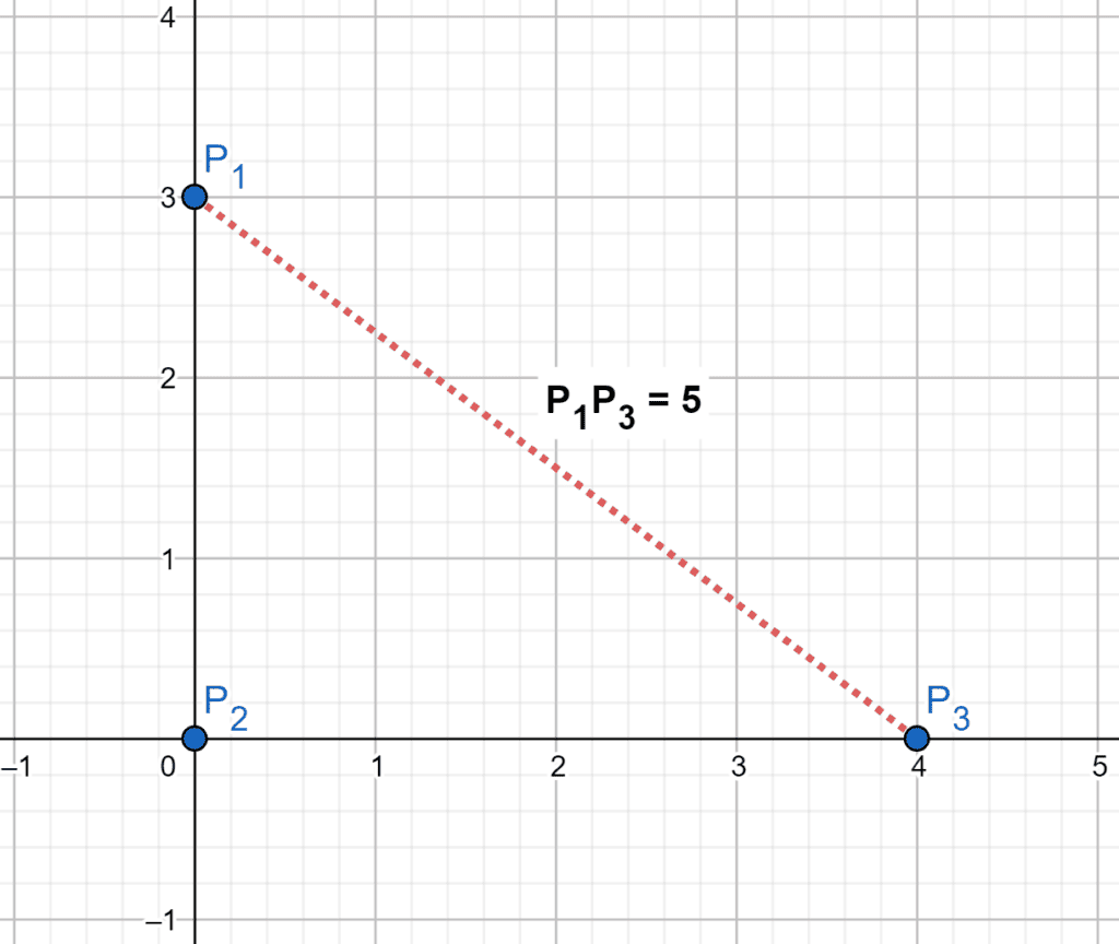We have three possible pair of points:

$P_1 - P_2$ with distance $3$ .
$P_1 - P_3$ with distance $5$ .
$P_2 - P_3$ with distance $4$ .

As we can see, the maximum distance is between points $P_1$ and $P_3$ , and it’s equal to $5$ .

3. Naive Approach

3.1. Main Idea

The main idea of this approach is to brute force all the possible pairs of points and get the pair with maximum distance.

Initially, we’ll go through every point that could potentially be the first point in the desired pair. Then, we try it with all the other points for each point. After that, for each pair, we try to maximize the maximum distance that we have so far with the distance between the points of the current pair.

Finally, the answer will equal the maximum distance between all possible pairs of points.

3.2. Algorithm

Let’s take a look at the implementation of the algorithm:

Initially, we declare the $MaximumDistance$ function that will return the maximum distance between all possible pairs of points. The function will have one parameter, $Points$ , representing the given set of points.

Next, we declare $answer$ , which will store the maximum distance, and initially, it equals $0$ . Then, we’ll brute force all possible pairs of points. For each point, we iterate over all other points and check the distance between the points of the current pair. If the distance is greater than the current $answer$ , we update $answer$ to equal the distance between the points of the current pair.

Finally, the $answer$ will equal the maximum possible distance between any pair of points.

3.3. Complexity

The time complexity of this algorithm is $\boldsymbol{O(N^2)}$ , where $N$ is the number of the given points. This complexity is because, for each point, we are iterating over all other points.

4. Rotate Calipers Approach

4.1. Main Idea

The main idea behind this approach is that the most distance pair of points will be from the vertices of the convex hull of the given set of points, and the maximum distance we could get is equal to the diameter of that convex polygon.

We’ll split this approach into two phases:

Convex Hull: we’ll build the convex hull of the given set of points since the desired pair of points will belong to the vertices of the convex hull. The reason behind that is if we take a line segment defined by a pair of points that lies inside the convex hull, we could extend the ends of that line segment to touch the boundary of the convex hull. Therefore, we’ll get a better solution.
Convex polygon diameter: the farthest pair of points we could get from the vertices of a convex polygon will be the pair of vertices that define the diameter of that polygon.

Therefore, the maximum distance is the length of the convex hull’s diameter formed from the given set of points.

4.2. Convex Hull

Let’s take a look at the implementation of building a convex hull algorithm:

Initially, we have the $ConvexHull$ function that will return the convex hull vertices defined by the given set of points. The function will have one parameter $Points$ represent the set of the given points.

First, we declare the $start\_ point$ , which will be the first vertex of the convex hull, and it’s equal to the point with the minimum value of x-coordinate since it’s an extreme point and we can guarantee that it’s from the convex hull vertices.

Second, we remove the $start\_ point$ from the $Points$ set, then we’ll sort the rest of the points with respect to the $start\_ point$ according to their slope:

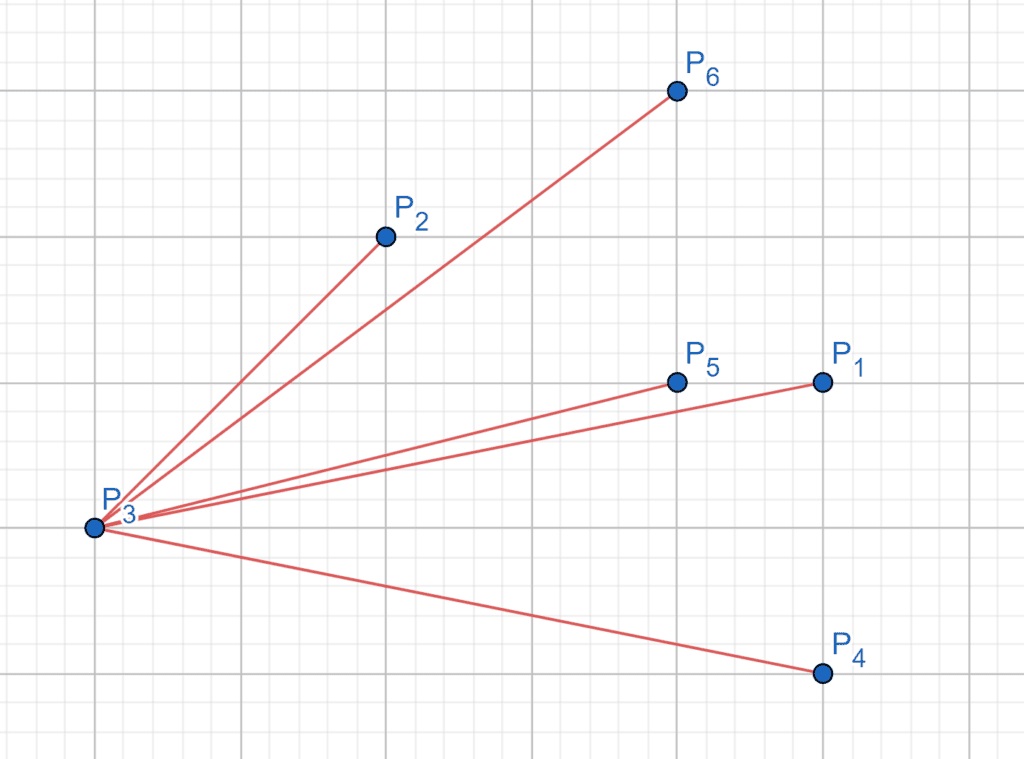
As we can see, the point $P_3$ is the $start\_ point$ since it’s the point with the minimum x-coordinate value, and the order of the rest of the points with respect to the $start\_ point$ according to their slopes will be $P_2 \rightarrow P_6 \rightarrow P_5 \rightarrow P_1 \rightarrow P_4$ .

Third, declare the $CH$ list, which will store the vertices of the convex hull. We add the $start\_ point$ to $CH$ since it’s from the convex hull vertices. Then, we iterate over the sorted points.

We’ll make two vectors. The first one represents the vector between the last two points in the current convex hull, and the other one will be between the point before the last and existing points. For each point, while we have at least two points in the convex hull, we want to check if the last point is one of the vertices of the convex hull or not.

If the cross-product of these two vectors is less than or equal to zero, we’ll make a right turn by adding the current point. So, the last point is valid, and we break out of the loop. Otherwise, we make a left turn, which means the current point is better than the last one. So, we pop the last point out of the $CH$ . In the end, we append the current point to the convex hull:

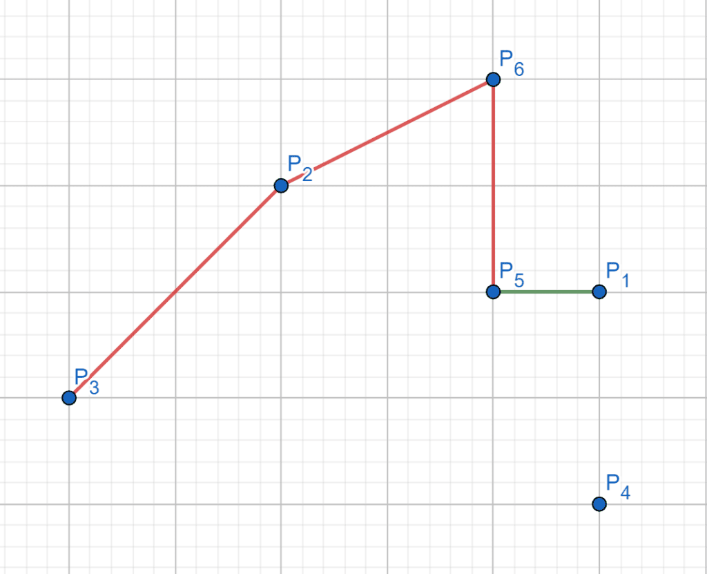
As we can see, the current $CH$ have points $P_3$ , $P_2$ , $P_6$ and $P_5$ . When we want to add $P_1$ to the convex hull, it will make a left turn with the last two points. Therefore, we pop the last point $P_5$ from the $CH$ .

Finally, the $CH$ will have the vertices of the convex hull sorted in clockwise order.

4.3. Convex Polygon Diameter

Let’s take a look at the implementation of the algorithm:

Initially, we have the $MaximumDistance$ function as the previous approach. The maximum distance will equal the diameter’s length of the convex hull. In addition, the length of the diameter is equal to the maximum value among all the antipodal pairs’ distances. (Recall a pair of polygon’s vertices $\boldsymbol{P}$ and $\boldsymbol{Q}$ called an antipodal pair if $\boldsymbol{P}$ and $\boldsymbol{Q}$ lie on parallel tangent lines of support).

First, we have $CH$ equal to the convex hull of the given points. Also, we declare $N$ , which is equal to the size of the convex polygon. Then, have a pointer $K$ , representing the position of the farthest point to the line segment defined by the first point and the last point of the convex polygon, which will be an antipodal point with the first point.

After that, we keep moving the $K$ pointer while the area of the $Triangle(CP[0], CP[N - 1], CP[K])$ is less than the area of $Triangle(CP[0], CP[N - 1], CP[K + 1])$ :

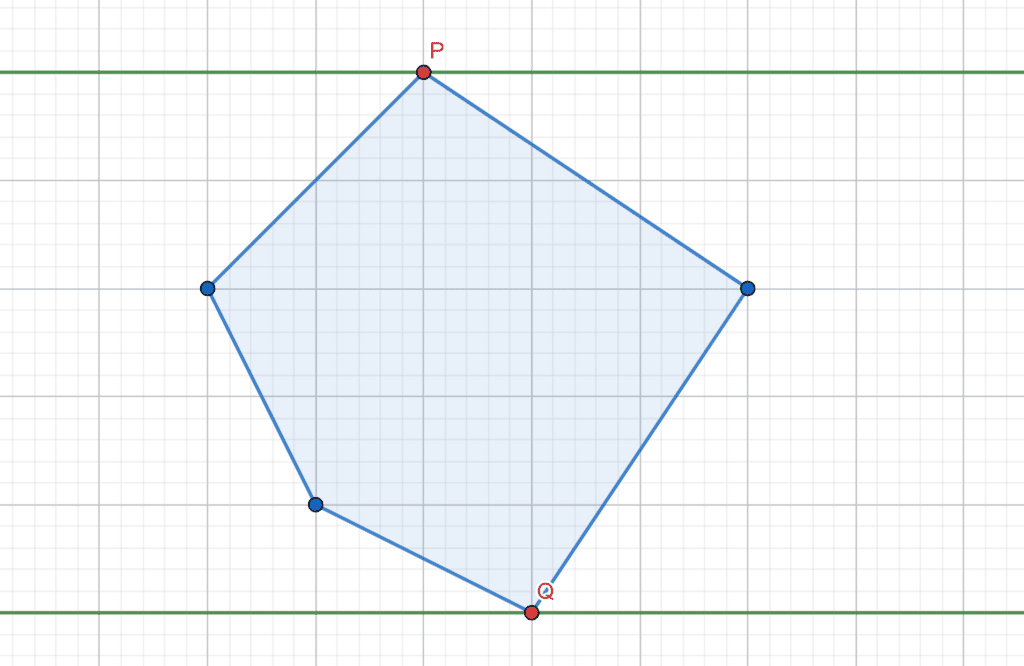
Second, we have an antipodal pair $P = 0$ and $Q = K$ , now we’ll use the rotate calipers technique to get all the antipodal pairs, while we’re moving the first pointer $P$ , we’ll keep moving $Q$ to be as far as possible from segment $CH[P], CH[P + 1]$ . If the distance between the current antipodal pair is greater than the current $answer$ , then we update the $answer$ to be equal to that value.

Finally, the $answer$ will equal the maximum possible distance between any pair of points.

4.4. Complexity

The time complexity of this algorithm is $\boldsymbol{O(N \times Log_2(N))}$ , where $N$ is the number of the given points. The reason behind this complexity is that the complexity of building the convex hull is $O(N \times Log_2(N))$ because we sort the points before building the convex hull.

Also, the time complexity of the rotate caliper technique is $O(N)$ because each of the two pointers will pass on the polygon vertices at most once. Thus, the total complexity of this approach is $O(N \times Log_2(N))$ .

5. Conclusion

In this article, we discussed the problem of finding the distance between the farthest pair of points from a given set of points. We provided an example to explain the problem and explored two different approaches to solve it, where the second one had a better time complexity.

Finally, we walked through their implementations and explained the idea behind each of them.

Full Archive

About Baeldung

Core Concepts

Operating Systems

Artificial Intelligence

Graph Theory

Latex