Finding the Minimum Number of Jumps to Reach the End of an Array

1. Overview

In this tutorial, we’ll talk about the problem of finding the minimum number of jumps to reach the end of a given array starting from the beginning.

First, we’ll define the problem and provide an example to explain it. Then, we’ll present three different approaches to solving it and work through their implementations and their space and time complexity.

2. Defining the Problem

Suppose we have an array $A$ of positive integers, where each element in that array represent the maximum length of the jump we can make to the right. We consider the end of the array as the position after the last element. We were asked to find the minimum number of jumps we could make starting from the first element to reach the end of the array.

Let’s take a look at the following example:

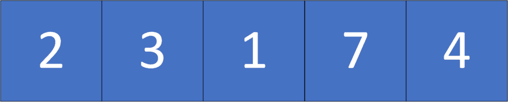
We can reach the end of the given array in multiple ways. Let’s take a look at a few of them:

$2 \rightarrow 1 \rightarrow 7 \rightarrow end$ .
$2 \rightarrow 3 \rightarrow 7 \rightarrow end$ .
$2 \rightarrow 3 \rightarrow end$ .

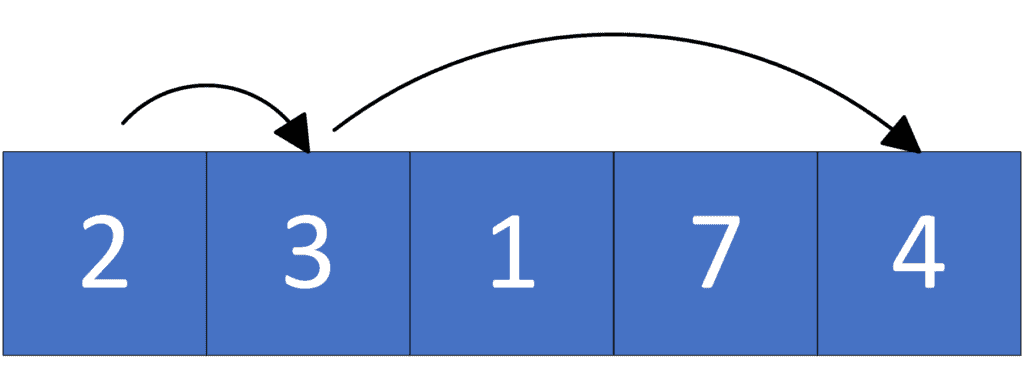
As we can see, the minimum number of jumps to reach the end of the given array is $2$ , where we take the path $2 \rightarrow 3 \rightarrow 4$ .

3. Naive Approach

3.1. Main Idea

The main idea in this approach is to try all possible solutions, then get the optimal solution with the minimum number of jumps.

Initially, we’ll have a recursive method to try all the possible solutions. We’ll try to jump to all viable cells from each position with a distance less than or equal to the current element value. Each time we make a call (jump), we increase the number of jumps by one.

Finally, we take the minimum value between all possible calls, representing the minimum number of jumps to reach the end of the given array starting from the current element.

3.2. Algorithm

Let’s take a look at the implementation of the algorithm:

Initially, we declare the $MinimumJumps$ function, which will try all possible solutions to reach the end of the given array. The function will have two parameters: The given array $A$ , and $index$ representing the current position in the array.

First, the base case of the recursive function here is when we reach the end of the array $A$ , then we return $0$ , the minimum number of jumps to reach the end of the given array starting from the end of the array.

Second, we declare $jumps$ , representing the minimum number of jumps to reach the end of the given array starting from the current position. Initially, its value equals infinity. Then we’ll take the minimum answer among all possible moves we can make. We’ll get the optimal answer for each possible next position starting from that position plus one, which represents the current jump.

Finally, the $MinimumJumps(A, 0)$ will return the minimum number of jumps to reach the end of the given array $A$ starting from the first element.

3.3. Complexity

The time complexity in the worst case is $\boldsymbol{O(M^N)}$ , where $N$ is the length of the given array $A$ , and $M$ is the maximum value inside the array. For each position in the array, we have $M$ choices, which represent the maximum length of jump we can make.

On the other hand, the space complexity of this algorithm is $\boldsymbol{O(1)}$ . The reason behind this complexity is that we use a single variable that equals the minimum number of jumps.

4. Dynamic Programming Approach

4.1. Main Idea

The main idea in this approach is the same as the previous one. However, since we have overlapping states, we can use dynamic programming.

Initially, the state of this dynamic programming approach will be $DP_i$ , which represents the minimum number of jumps to reach the end of the array starting from the position $i$ . Next, since the answer of each state depends on the answers of the next ones, we’ll start calculating the answer of each state starting from the end towards the beginning. Then, for each state $i$ , we’ll take the minimum value among all states solution in range $[i + 1, i + A_i]$ .

Finally, the $DP_0$ will represent the minimum number of jumps to reach the end of the given array starting from the first position.

4.2. Algorithm

Let’s take a look at the implementation of the algorithm:

Initially, we have the $MinimumJumps$ function as the previous approach. It has one parameter $A$ , which represents the given array.

First, we declare the $DP$ array, which will store the minimum number of jumps to reach the end of the array $A$ starting from each position.

Second, we set the value of $DP[ length(A) ]$ to $0$ , which represents the minimum number of jumps to reach the end starting from the end. Next, for each position from the end towards the beginning, we’ll try to jump to the cell with the minimum answer among all the cells in the range $[i + 1, i + A_i]$ .

Finally, the $DP[0]$ will have the minimum number of jumps to reach the end of the given array $A$ starting from the first element.

4.3. Complexity

The time complexity of this algorithm is $\boldsymbol{O(N \times M)}$ , where $N$ is the length of the given array $A$ , and $M$ is the maximum length of a jump. The reason behind this complexity is that for each position, we try to make all possible jumps.

The space complexity of this algorithm is $\boldsymbol{O(N)}$ , where $N$ is the length of the given array $A$ . The reason is that we store the minimum number of jumps for each position.

5. Greedy Approach

5.1. Main Idea

The main idea in this approach is to keep moving forward as long as we can. The moment we can’t move, we’ll jump from the cell that takes us as far as possible among all the cells that we’ve passed through.

Initially, in this approach, we care about two things:

Maximum reachability: This represents the maximum position we can reach using one of the jumps that we have iterated through.
Moves: The number of moves we can make using the last jump we’ve made.

Next, while iterating over the array, we’ll update the maximum position we can reach and decrease the number of moves by one. The moment we run out of moves, we’ll jump from the cell that allows us to reach the maximum position, and we’ll increase the number of jumps by one.

In the end, the number of jumps will be the optimal solution that we could make, and it’ll be the answer to the problem.

5.2. Algorithm

Let’s take a look at the implementation of the algorithm:

Initially, we have the $MinimumJumps$ function similarly to the previous approaches.

First, we declare the $maxReach$ variable, which will store the maximum position we can reach using the cells that we’ve passed through. Initially, it’s equal to the first element.

Also, We declare the $moves$ variable, which stores the maximum number of moves we could make using the last jump. Its initial value equals the first element as well. In addition, we declare $jumps$ , which will store the number of jumps we made so far and initially equal one representing the jump from the first element.

Second, we loop through the elements of the given array. In each iteration, we’ll maximize $maxReach$ with the next position that uses the maximum length of the current jump. Also, we’ll decrease the number of moves we can make by one. After that, we check whether we run out of $moves$ . If so, we’ll make a jump using the cell that gets us to the $maxReach$ position.

Furthermore, the new value of $moves$ will equal $maxReach - i$ , because we decide to use the best jump, which should make us reach the $maxReach$ position, which needs $maxReach - i$ moves from our current position.

Finally, the $jumps$ will have the minimum number of jumps we need to reach the end of the array $A$ starting from the first element.

5.3. Complexity

The time complexity of this algorithm is $\boldsymbol{O(N)}$ , where $N$ is the length of the given array $A$ . This complexity is because we iterate over each position only once.

The space complexity of this algorithm is $\boldsymbol{O(1)}$ . The reason is that we have a constant number of variables.

6. Conclusion

In this article, we discussed the problem of finding the minimum number of jumps to reach the end of an array. First, we provided an example to explain the problem. Then, we explored three different approaches to solving it, where each one of them had a better time complexity than the previous one.

Finally, we walked through their implementations and explained the idea behind each of them.

Full Archive

About Baeldung

Core Concepts

Operating Systems

Artificial Intelligence

Graph Theory

Latex

1. Overview

2. Defining the Problem

3. Naive Approach

3.1. Main Idea

3.2. Algorithm

3.3. Complexity

4. Dynamic Programming Approach

4.1. Main Idea

4.2. Algorithm

4.3. Complexity

5. Greedy Approach

5.1. Main Idea

5.2. Algorithm

5.3. Complexity

6. Conclusion