Greedy Algorithm to Find Minimum Number of Coins

1. Introduction

In this tutorial, we’re going to learn a greedy algorithm to find the minimum number of coins for making the change of a given amount of money. Usually, this problem is referred to as the change-making problem.

At first, we’ll define the change-making problem with a real-life example. Next, we’ll understand the basic idea of the solution approach to the change-making problem and illustrate its working by solving our example problem.

Then, we’ll discuss the pseudocode of the greedy algorithm and analyze its time complexity. Finally, we’ll point out the limitation of the discussed algorithm and suggest an alternative to overcome it.

2. Change Making Problem

In the change-making problem, we’re provided with an array = of distinct coin denominations, where each denomination has an infinite supply. We need to find an array having a minimum number of coins that add up to a given amount of money , provided that there exists a viable solution.

Let’s consider a real-life example for a better understanding of the change-making problem.

Let’s assume that we’re working at a cash counter and have an infinite supply of valued coins. Now, we need to return one of our customers an amount of using the minimum number of coins.

3. Solution Approach

The greedy algorithm finds a feasible solution to the change-making problem iteratively.

At each iteration, it selects a coin with the largest denomination, say , such that . Next, it keeps on adding the denomination to the solution array and decreasing the amount by as long as . This process is repeated until becomes zero.

Let’s now try to understand the solution approach by solving the example above. The image below shows the step-by-step solution to our problem:

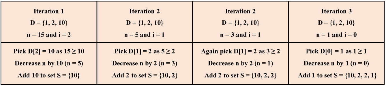
Hence, we require a minimum of four coins to make the change of amount , and their denominations are .

4. Pseudocode 

Now that we know the basic idea of the solution approach, let’s take a look at the pseudocode of the algorithm:

algorithm findMinimumNumberOfCoins(D, m, n):
    // INPUT
    //   D = The array of coin denominations
    //   m = The number of coin denominations
    //   n = The given amount of money
    // OUTPUT
    //   S = The array having minimum number of coins

    Sort the array D in ascending order of coin denominations

    S <- an empty array

    for i <- m - 1 to 0:
        while n >= D[i]:
            S <- append D[i] to S
            n <- n - D[i]

        if n = 0:
            break

    return S

To begin with, we sort the array of coin denominations in ascending order of their values.

Next, we start from the last index of the array and iterate through it till the first index. At each iteration, we add as many coins of each denomination as possible to the solution array and decrement by the denomination for each added coin.

Once becomes zero, we stop iterating and return the solution array as an outcome.

Let’s now analyze the time complexity of the algorithm above.

We can sort the array of coin denominations in () time. Similarly, the for loop takes () time, as in the worst case, we may need coins to make the change.

Hence, the overall time complexity of the greedy algorithm becomes () since . Although, we can implement this approach in an efficient manner with () time.

5. Limitation

The limitation of the greedy algorithm is that it may not provide an optimal solution for some denominations.

For example, the above algorithm fails to obtain the optimal solution for and . In particular, it would provide a solution with four coins, i.e., .

However, the optimal solution for the said problem is three coins, i.e., .

The reason is that the greedy algorithm builds the solution in a step-by-step manner. At each step, it picks a locally optimal choice in anticipation of finding a globally optimal solution. As a result, the greedy algorithm sometimes traps in the local optima and thus could not provide a globally optimal solution.

As an alternative, we can use a dynamic programming approach to ascertain an optimal solution for general input. In fact, we’ll discuss the dynamic programming-based algorithm in some other article.

6. Conclusion

In this article, we’ve studied a greedy algorithm to find the least number of coins for making the change of a given amount of money and analyzed its time complexity. Further, we’ve also illustrated the working of the discussed algorithm with a real-life example and discussed its limitation.