Maximum Single-Sell Profit | Baeldung on Computer Science

1. Overview

In this tutorial, we’ll discuss the problem of finding the Maximum single-sell profit in an array. We’ll present a naive approach and then improve it to obtain a better solution.

2. Defining the Problem

Suppose we’re concerned with a product. In advance, we know the prices of this product over the next $n$ days. The price of the i^th day is denoted as $P_i$ . Hence, we’re given an array called $P$ of size $n$ .

We must choose two days from this array. On the first day, we’ll buy the product, and on the second, we’ll sell it. We need to make the maximum profit from this operation.

In other words, we need to find the maximum value of $P_j - P_i$ , such that $j \geq i$ .

3. Naive Approach

First, we’ll explore the naive approach. Let’s take a look at its implementation:

algorithm MaxSingleSellProfitNaive(P, n):
    // INPUT
    //     P = the prices array
    //     n = the size of the prices array
    // OUTPUT
    //     maximum single-sell profit, buy day, and sell day

    Answer <- 0
    buyDay <- 0
    sellDay <- 0
    for i <- 1 to n:
        for j <- i to n:
            if Answer <= P[j] - P[i]:
                Answer <- P[j] - P[i]
                buyDay <- i
                sellDay <- j

    return Answer, buyDay, sellDay

In this approach, we’re checking all possible values of $P_j - P_i$ . Hence, we call this the brute force approach.

We iterate over all possible pairs $i$ and $j$ , such that $j$ always starts from $i$ and moves forward. The index $i$ represents the day we buy the product. On the other hand, the index $j$ represents the day we sell the product.

Therefore, $j$ starts from $i$ and moves forward because we can’t sell a product if we haven’t bought it yet.

For each pair ( $i$ , $j$ ), we check whether we can get a better profit from the already found profit. If so, we update the stored profit. Also, we store the day we decided to buy the product and the day we decided to sell it.

In the end, we return the stored answer and both indexes of the days to buy and sell the product in.

The complexity of the naive approach is $O(n^2)$ , where $n$ is the number of days.

4. Dynamic Programming Approach

Let’s try to improve our naive approach.

4.1. General Idea

In the naive approach, we tried all possible pairs of days $i$ and $j$ . However, if we think deeply, we can see that when we decide to sell a product on the day $j$ , it’s always optimal to choose the smallest price in days $[1..j]$ to buy the product in before selling it.

So, in each step, we need to calculate the value $lowest$ , which stores the smallest value before, and including, the current index $j$ . Let’s use dynamic programming to calculate the values $lowest$ quickly.

Suppose we calculated the lowest price values before the index $j$ , and we need to calculate the value when we reached the index $j$ . The first solution would be to iterate over all the values in range $[1, j]$ and take the minimum value among them.

However, we can notice that the previous value of $lowest$ represents the range $[1, j - 1]$ . Since the current range is $[1, j]$ , we can see that it differs only by the index $j$ from the previous range.

Thus, we can simply calculate the minimum value in range $[1, j]$ by taking the minimum between the previous value of $lowest$ and $P[j]$ .

Let’s take the following example to explain the idea better:

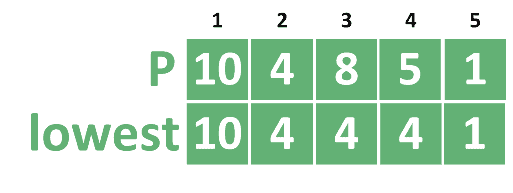
First of all, we assign $lowest = P[1] = 10$ because we don’t have a previous range yet. After that, for each index $j$ we take the minimum between the previous value of $Lowest$ and $P[j]$ .

Now that we showed how to calculate the $lowest$ values, we can use it to improve the naive approach.

4.2. Implementation

Take a look at the implementation of the dynamic programming approach:

algorithm MaxSingleSellProfitDP(P, n):
    // INPUT
    //     P = the prices array
    //     n = the size of the prices array
    // OUTPUT
    //     The maximum single-sell profit, buy day, and sell day

    indexOfLowest <- 0
    Lowest <- P[0]
    Answer <- 0
    buyDay <- 0
    sellDay <- 0
    for j <- 1 to n:
        if P[j] <= Lowest:
            indexOfLowest <- j
            Lowest <- P[j]
        if Answer <= P[j] - Lowest:
            Answer <- P[j] - Lowest
            buyDay <- indexOfLowest
            sellDay <- j

    return Answer, buyDay, sellDay

Instead of calculating an entire array $lowest$ , we’ll just keep a variable named $lowest$ , that stores the minimum value so far.

In each step, we check if the current value is smaller than the lowest price so far. If so, we update the value of $indexOfLowest$ and $Lowest$ . Note that we’ll store the index of the minimum value to be able to determine the day that we should buy the product in.

After that, we check whether the current selling day with the lowest buying day gives a better solution than the stored one. If so, we store the profit we get as the best one so far. Also, we’ll store the index $indexOfLowest$ as the buying day and index $j$ as the selling day.

Finally, we return the stored answer and both indexes of the buying and selling days.

The complexity of this approach is $O(n)$ , where $n$ is the number of days.

5. Conclusion

In this tutorial, we explained the problem of finding the maximum single-sell profit from an array of prices. In the beginning, we presented the naive approach. Then, we showed how to improve it to obtain a dynamic programming solution.

Full Archive

About Baeldung

Core Concepts

Operating Systems

Artificial Intelligence

Graph Theory

Latex