Yes, we're now running our only Summer Sale. All Courses are 30% off until 20th July, 2026:
Error Detection: Hamming Code
Last updated: June 21, 2023

Learn through the super-clean Baeldung Pro experience:
>> Membership and Baeldung Pro.
No ads, dark-mode and 6 months free of IntelliJ Idea Ultimate to start with.
1. Introduction
Error detection and correction are crucial to ensure reliable data transmission between devices. One of the most widely used error detection and correction methods is Hamming code. Richard Hamming developed it in 1950 at Bell Labs. In particular, it can detect and correct a single-bit error by adding redundant (or parity) bits to the original data.
A few use cases of Hamming code include:
-
- Computer memory systems: RAM and hard disk
- Communication networks: Bluetooth, ethernet, and wi-fi
- Digital signal processing: Satellite communications and digital audio broadcasting
In this tutorial, we’ll first study the basic terms of Hamming code, such as redundant bits, parity bits, and parity bit calculation. Next, we’ll provide an illustrative example of how to encode a data block using the Hamming code. Then, we’ll explore the various steps involved in error detection and correction. After that, we’ll discuss the advantages and limitations of the Hamming code. Finally, we’ll wrap up the tutorial with a brief summary of the topics covered.
2. Hamming Code Basics
In this section, we’ll discuss the fundamental terminologies of the Hamming code, including redundant bits, parity bits, and parity bit calculation.
2.1. Redundant Bits
The central idea of the Hamming code is based on redundancy. In general, the sender first divides the original data into fixed-sized blocks. It then adds some extra redundant bits to each data block before transmitting the block to the receiver. Upon reception, the receiver uses these bits to detect transmission error, locate the corrupted bit, and correct it. We can calculate the required number of redundant bits using the equation:
![\[ 2^R \geq M + R + 1\]](/wp-content/ql-cache/quicklatex.com-a63b72bf7cfb45c5172d24f3082688d8_l3.svg "Rendered by QuickLaTeX.com")
In this equation,  is the number of redundant bits, and
  is the number of data bits in a block.
2.2. Parity Bits
We add parity bits as redundant bits to an original data block for detecting and correcting errors during transmission. These bits ensure that each data block’s total count of  is either even or odd. There are two types of parity bits:
Odd parity bit: We set a parity bit to when the count of in a bit sequence is even; otherwise, we configure it to  .
.
Even parity bit: We fix a parity bit to if the count of in a given set of bits is odd; otherwise, we set it to .
2.3. Parity Bit Calculation
A Hamming code has  number of bits, which is the sum of data bits and parity bits. We now discuss the step-by-step process to obtain the position and value of parity bits:
- At first, we compute the number of parity bits using
 and the total number of bits in the Hamming code using
- Next, we convert the bit positions from to into binary numbers, i.e.,
![[0001,0010,0011,0100, 0101, 0110, 0111,1000,\cdots]](/wp-content/ql-cache/quicklatex.com-0cf4b82b434bf8e58c261105184aa5cc_l3.svg "Rendered by QuickLaTeX.com")
- Then, we label the bit positions corresponding to the power of
 as parity bits and the remaining positions as the data bits, e.g.,
 ![[P_1,P_2,D_1,P_3, D_2, D_3, D_4,P_4,\cdots]](/wp-content/ql-cache/quicklatex.com-83b8fcc894b9b94e0d14757f4020ea59_l3.svg "Rendered by QuickLaTeX.com")
- At last, we determine the value of each parity bit in the Hamming code iteratively. In each iteration, we determine the value of parity bit
 by counting the number of in the bit positions that have in the
  position from the least significant bit in their binary representations. Then, we set the parity bit to if the number of is odd, considering even parity; otherwise, we set it to
3. An Illustrative Example
Let’s break down the process of generating a Hamming code by looking at an example binary data block  . This will help us understand how the Hamming code works and how it detects and corrects errors during data transmission. We’ll now apply each of the steps discussed in the previous section, one by one.
Step 1: The number of parity bits is  since
since  and
and  . Therefore, the length of the Hamming code is
  , that is,
  .
.
Step 2: The binary conversion of the bit positions from to  is
is ![[0001,0010,0011,0100, 0101, 0110, 0111,1000,1001,1010,1011,1100,1101,1110,1111]](/wp-content/ql-cache/quicklatex.com-7c63ba8be5ecb03e8ca9b4f3bc66108a_l3.svg "Rendered by QuickLaTeX.com") .
.
Step 3: The parity bits are placed at the positions ![[1,2,4,8]](/wp-content/ql-cache/quicklatex.com-c088f6a621b422eb11835967aa677124_l3.svg "Rendered by QuickLaTeX.com") since they are power of . In contrast, the data bits are kept at the positions
since they are power of . In contrast, the data bits are kept at the positions ![[3,5,6,7,9,10,11,12,13,14,15]](/wp-content/ql-cache/quicklatex.com-9ee9963f10a95f7301b3fd78bfd7d443_l3.svg "Rendered by QuickLaTeX.com") . The image below shows the labeling of parity and data bits:
. The image below shows the labeling of parity and data bits:
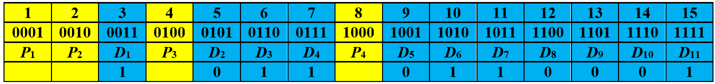
Step 4 – iteration 1: In the first iteration, we calculate the value of parity bit  by counting the number of at the positions
 ![[1,3,5,7,9,11,13,15]](/wp-content/ql-cache/quicklatex.com-898aa183bfc436e748956a3b9620ace5_l3.svg "Rendered by QuickLaTeX.com") . These positions are chosen because their first bit from the least significant bit is equal to 1 in their binary representations. It is illustrated by:
. These positions are chosen because their first bit from the least significant bit is equal to 1 in their binary representations. It is illustrated by:
by counting the number of at the positions . These positions are chosen because their first bit from the least significant bit is equal to 1 in their binary representations. It is illustrated by: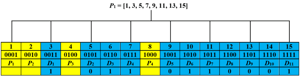
We consider even parity and set the parity bit  since the count of at the positions is
  . The updated code is:
since the count of at the positions is . The updated code is: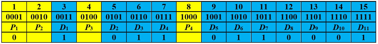
Step 4 – iteration 2: Next, the value of parity bit  is calculated based on the number of at the positions
 ![[2, 3, 6, 7, 10, 11, 14, 15]](/wp-content/ql-cache/quicklatex.com-ebb56c91c4a058682755544af4e5526d_l3.svg "Rendered by QuickLaTeX.com") . This is because the second bit from the least significant bit of these positions are 1 in their binary representations:
. This is because the second bit from the least significant bit of these positions are 1 in their binary representations:
is calculated based on the number of at the positions . This is because the second bit from the least significant bit of these positions are 1 in their binary representations: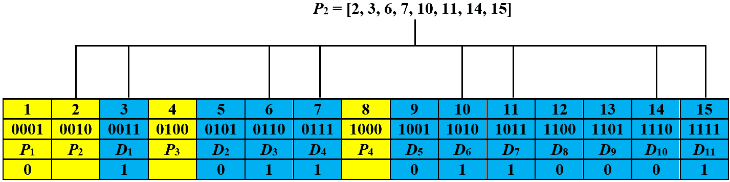
We then assign  because there are
  occurrences of at the positions . The new code is:
because there are occurrences of at the positions . The new code is: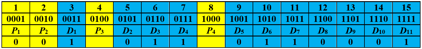
Step 4 – iteration 3: In the third iteration, we calculate the value of parity bit  . To do so, we first count the number of at the positions
 ![[4, 5, 6, 7, 12, 13, 14, 15]](/wp-content/ql-cache/quicklatex.com-e5fd05fc72926bd70071fae2b0317410_l3.svg "Rendered by QuickLaTeX.com") . The reason is that the third bit from the least significant bit in the binary representation of these positions is . It can be seen in the image below.
. The reason is that the third bit from the least significant bit in the binary representation of these positions is . It can be seen in the image below.
. To do so, we first count the number of at the positions . The reason is that the third bit from the least significant bit in the binary representation of these positions is . It can be seen in the image below.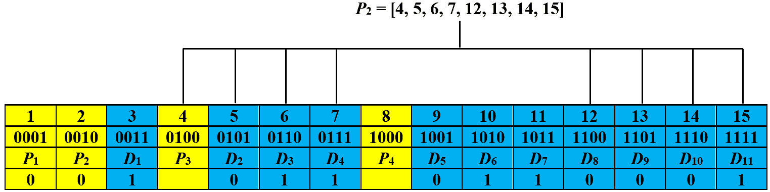
Next, we set the value of parity bit  because we count
  instances of at the positions . Now, the code is:
because we count instances of at the positions . Now, the code is: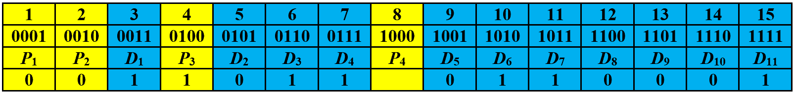
Step 4 – iteration 4: We finally count the number of at the positions ![[8,9,10,11,12,13,14,15]](/wp-content/ql-cache/quicklatex.com-9802832c4e84620cebcc480237716cf6_l3.svg "Rendered by QuickLaTeX.com") to finalize the value of parity bit
to finalize the value of parity bit  . This is because the fourth bit from the least significant bit is equal to 1 in the binary representation of these positions:
at the positions to finalize the value of parity bit . This is because the fourth bit from the least significant bit is equal to 1 in the binary representation of these positions: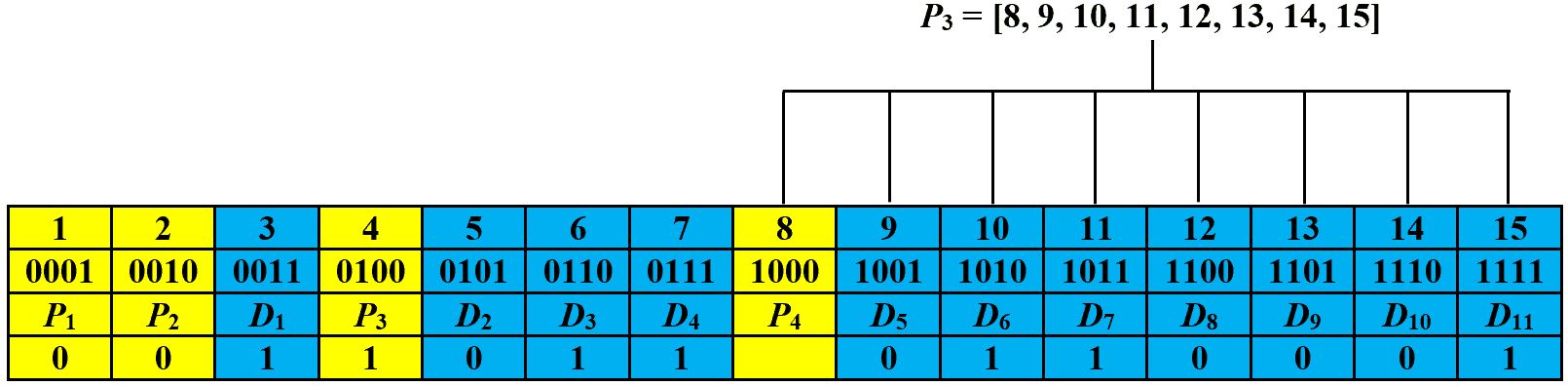
Hence, we set the parity bit  since the count of at the positions is . The final Hamming code is:
since the count of at the positions is . The final Hamming code is: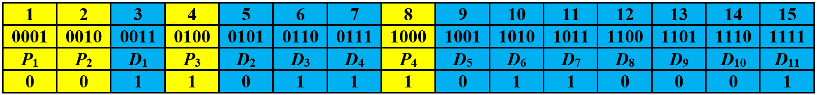
4. Error Detection and Correction
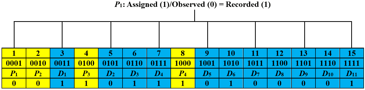
Let’s first discuss how to detect if there is an error in the received code. To do so, we recalculate the values of parity bits and perform parity checks. In particular, we record a for a parity check if the assigned and observed parity bits do not match. Otherwise, we record a . The recorded values are then written from right to left to form the checking number. The code is error-free if the checking number is zero. Otherwise, an error has occurred at the bit position corresponding to the checking number, given that there is only a single-bit error.
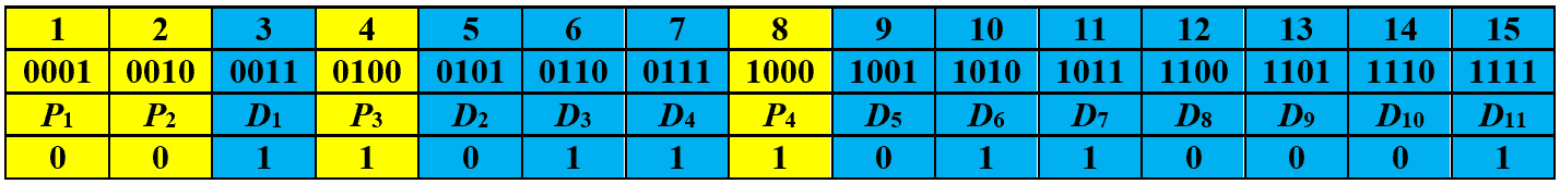
Let’s assume that the eleventh bit of the codeword generated in the previous section is changed from to during transmission. Then, the received code is:
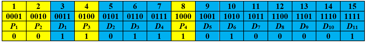
Now, we recalculate the parity bits and record their values based on the assigned and observed parity bits. The images below show the recorded values for parity bits , , , and , respectively:
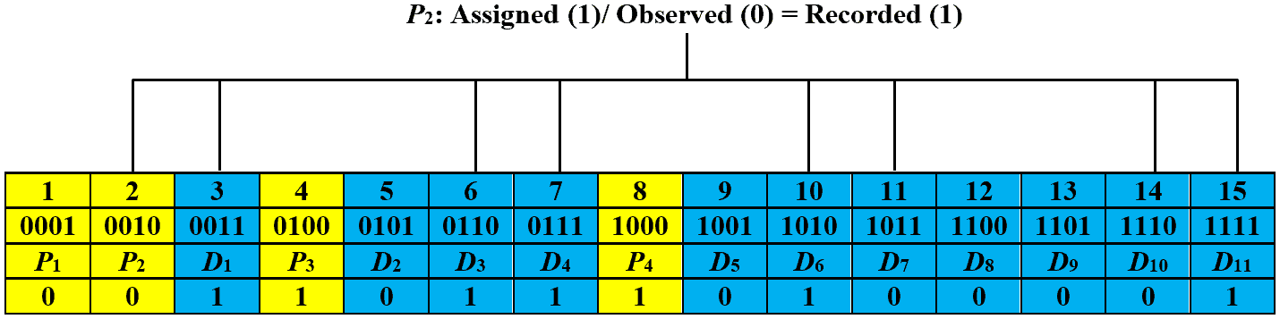
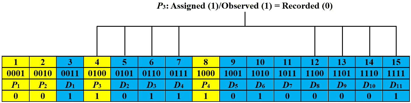
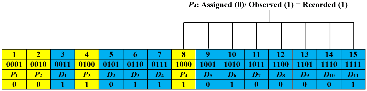
Let’s obtain the checking number by writing the recorded values from right to left, i.e.,  , which is equal to decimal number eleven. This signifies that the received code has an error at the eleventh bit. In order to correct it, we just have to toggle the eleventh bit and the corrected code is:
5. Advantages and Limitations
The key advantages and notable limitations of the Hamming code are:
| Advantages | Limitations |
|---|---|
| 1. Hamming code is easy to understand and implement. | 1. Hamming code can detect and correct only single-bit errors. |
| 2. It can efficiently detect and correct single-bit errors in data without the need for retransmission. | 2. The addition of redundant bits increases the size of the data block and reduces the efficiency of transmission. |
| 3. Hamming code is a cost-effective method as it does not require expensive hardware or software. | 3. The fixed block size of the Hamming code may not be suitable for applications with variable data size. |
| 4. It can be adapted to work with different block sizes, making it a versatile solution for error detection and correction. | 4. It may not be flexible enough to handle different error patterns or positions within the codeword. |
6. Conclusion
This tutorial first provides a brief overview of the Hamming code and its use cases. It then explains the basic concepts of the Hamming code, such as redundant bits, parity bits, and parity bit calculation.
Next, it presents an illustrative example of encoding a data block using parity bits. Later, it discusses and demonstrates the steps involved in error detection and correction. In the end, it highlights the key advantages and limitations of the Hamming code.