Gray Code vs Natural Binary Representation | Baeldung on Computer Science

1. Overview

The natural binary representation assigns each binary digit a value of 0 or 1 based on powers of 2, allowing for straightforward arithmetic and logic operations. Essentially, it’s the mathematical representation of base-2 numbers. However, this representation faces challenges that the Gray code can address.

In this tutorial, we’ll explore the differences between Gray code and natural binary representation.

2. Historical Context and Motivation Behind Gray Code

In the early 20th century, mechanical and electromechanical systems, such as rotating machinery and switches, were prone to errors during state transitions. These errors occurred because the natural binary representation could cause multiple bits to change simultaneously, resulting in ambiguous or incorrect readings.

For example, in natural binary, the transition from 0111 (7) to 1000 (8) involves changing all four bits simultaneously, increasing the likelihood of misreading intermediate states. If an error occurs during this transition, the resulting value could be far from the intended value, making error detection and correction very complex.

Frank Gray’s 1947 introduction of Gray code addresses this problem by ensuring that only a bit changes during transitions between successive values. This single-bit change property reduces the potential for error, making Gray code particularly useful in applications where precise and reliable state changes are critical.

Another important motivation for Gray code is its potential to simplify error detection and correction in digital communication systems.

3. Definition and Key Characteristics

Let ${\mathcal S}^{ ( n ) }$ denote the set of all binary strings of length $n$ , where $N = 2^n$ . A Gray code of order $n$ is a sequence $S_0, S_1, \ldots, S_{N-1}$ of elements in ${\mathcal S}^{ ( n ) }$ such that every successive pair $(S_i, S_{i+1})$ of bitstrings differs by exactly one bit.

Here are its key features:

The standard implementation of Gray code is cyclic, i.e., $S_0$ and $S_{N-1}$ differ by exactly one bit
Gray code isn’t a weighted code, meaning there’s no direct relationship between a bit’s value (weight) and its position in the number
No known method directly converts a base-10 number to Gray code, or vice versa, without the intermediate conversion to natural binary representation
Gray code handles only non-negative integers

Let’s look at two examples of Gray code sequences:

2-bit Gray code: 00, 01, 11, 10
3-bit Gray code: 000, 001, 011, 010, 110, 111, 101, 100

Gray code is also known as reflected binary code (RBC).

4. Natural Binary vs. Gray Code

A notable early application was Gray code rotary encoders, which are still in use today. These devices convert the angular position or motion of a shaft or axis into digital output signals.

Here is an example of a 4-bit encoder that can measure 16 positions, each represented by a 4-bit Gray code. It consists of concentric circles, where each ring represents a different bit in the 4-bit code, starting from the innermost ring (most significant bit, MSB) to the outermost ring (least significant bit, LSB). The color-coded cells represent bit 0, while the white cells represent ones:

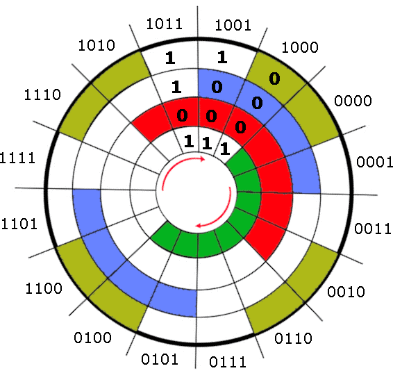
This encoder demonstrates a complete (clockwise) cycle from 0000 (0) to 1000 (15), highlighting the cyclic nature of Gray code. Each number differs from its predecessor in a single bit, unlike in the natural binary representation:

Position	Gray code	Natural binary
0	0000	0000
1	0001	0001
2	0011	0010
3	0010	0011
4	0110	0100
5	0111	0101
6	0101	0110
7	0100	0111
8	1100	1000
9	1101	1001
10	1111	1010
11	1110	1011
12	1010	1100
13	1011	1101
14	1001	1110
15	1000	1111

Gray code’s single-bit change property minimizes error risk, leading to its widespread adoption in various electromechanical systems.

5. Conversion Techniques

Before we continue, we need to know how to convert a number from base 10 to base 2 and what the XOR $\boldsymbol{\oplus}$ logic gate is.

5.1. Binary to Gray Code Conversion

We can convert a binary number $B = B_{n-1} B_{n-2} \ldots B_1 B_0$ to a Gray code number $G = G_{n-1} G_{n-2} \ldots G_1 G_0$ using this functional relationship:

$G_i = \begin{cases} B_i & \text{if } i = n-1 \\ B_{i+1} \oplus B_i & \text{if } 0 \leq i < n-1 \end{cases}$

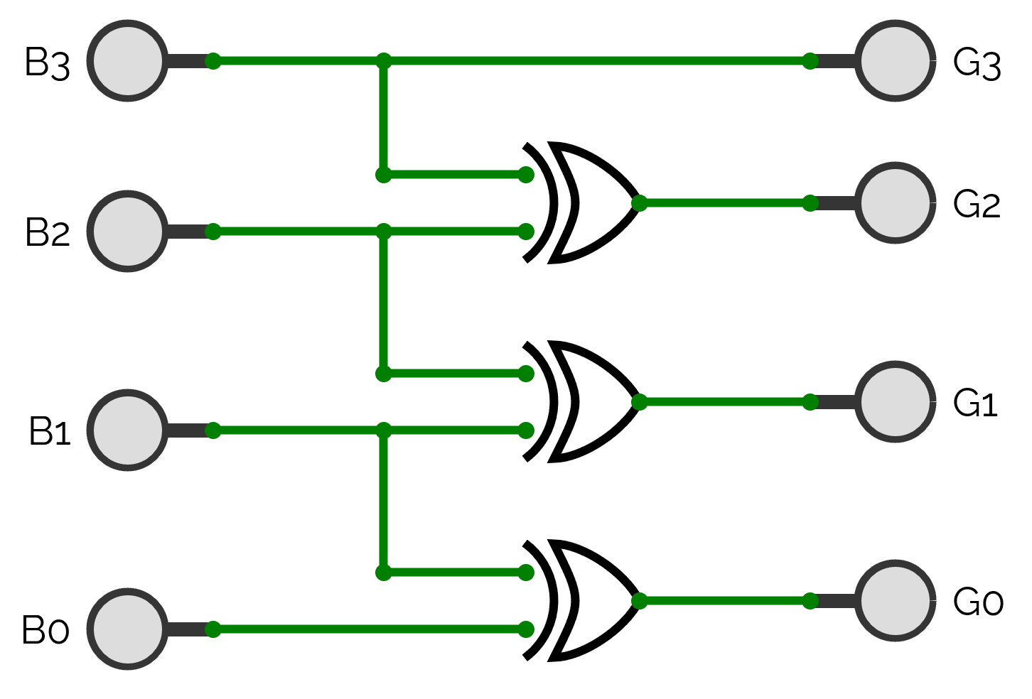
We can implement it with a logic circuit. Here’s how it looks for 4-bit numbers:

For example, let’s consider the 4-bit binary number $B = 1010$ :

$G_3 = B_3 = 1$
$G_2 = B_3 \oplus B_2 = 1 \oplus 0 = 1$
$G_1 = B_2 \oplus B_1 = 0 \oplus 1 = 1$
$G_0 = B_1 \oplus B_0 = 1 \oplus 0 = 1$

Thus, 1010 in binary converts to 1111 in Gray code.

5.2. Gray Code to Binary Conversion

We can convert a Gray code number $G = G_{n-1} G_{n-2} \ldots G_1 G_0$ to a binary number $B = B_{n-1} B_{n-2} \ldots B_1 B_0$ as follows:

$B_i = \begin{cases} G_i & \text{if } i = n-1, \\ B_{i+1} \oplus G_i & \text{for } 0 \leq i < n-1 \end{cases}$

Here’s how a circuit can do the conversion of four bits:

For example, let’s consider the 4-bit Gray code number $G = 1111$ :

$B_3 = G_3 = 1$
$B_2 = B_3 \oplus G_2 = 1 \oplus 1 = 0$
$B_1 = B_2 \oplus G_1 = 0 \oplus 1 = 1$
$B_0 = B_1 \oplus G_0 = 1 \oplus 1 = 0$

It maps to 1010 in binary.

6. Practical Applications

To better understand the differences between Gray code and natural binary code, here is a table comparing their properties in some practical applications:

Feature	Gray Code Advantage	Natural Binary Issue
Error Rate	Low due to single-bit transitions	High, as multiple bits may change simultaneously
Application in rotary encoders	High precision and reliability in position encoding	Prone to errors in fast or complex mechanical settings
Usage in analog to digital converters (ADCs)	Accurate analog to digital conversions	Increased potential for sampling errors
Robustness in digital communication	Improved signal integrity, especially under noisy conditions	Susceptibility to errors increases with noise and signal degradation
Implementation complexity	Simplifies circuit design for error checking and correction	Complex circuitry needed to manage and correct multiple bit changes
Implementation in visual display units (digital clocks, public information displays, etc.)	Consistent and error-free transitions ensure reliable data display	Possibility of flickering or incorrect display during transitions
Quantum computing	Potential for error reduction in qubit representation and manipulation	Less suitable due to high sensitivity to state changes

These advanced applications illustrate the broad utility of Gray code and demonstrate its potential in cutting-edge technology sectors.

7. Conclusion

In this article, we explored the basic concepts and practical applications of Gray code. The main difference between Gray code and natural binary representation is how they handle sequential numbers.

In natural binary representation, multiple bits can change simultaneously between two successive numbers, potentially causing errors in digital systems. In contrast, Gray code is designed so only a single bit changes between successive values, reducing the risk of errors during transitions.

Core Concepts

Operating Systems

Artificial Intelligence

Graph Theory

Latex

Full Archive

About Baeldung