

Learn through the super-clean Baeldung Pro experience:
>> Membership and Baeldung Pro.
No ads, dark-mode and 6 months free of IntelliJ Idea Ultimate to start with.
Last updated: March 18, 2024
Learn through the super-clean Baeldung Pro experience:
>> Membership and Baeldung Pro.
No ads, dark-mode and 6 months free of IntelliJ Idea Ultimate to start with.
In this tutorial, we’ll explore a few techniques for the procedural generation of maps, such as in a computer game. These are maps that are entirely random and so give much better variety for gameplay, and yet are still relatively realistic.
Many times in computer games, we want to give the impression of significantly more content than we can actually produce or store. Either because of restrictions in the production of the content in the first place – e.g. for a small production team – or else in the storage or distribution of the content.
We can get around this, though, with Procedural Generation. This is when the game generates new content on the fly at runtime instead of only using previously produced content. Done right, this can give us effectively limitless content in our game with much lower production costs up-front.
All procedural generation depends on being able to reliably produce random numbers. Depending on the exact need, we might also need to be able to produce the same sequence of random numbers over and over – i.e. use the same starting seed and the same algorithm to give the same stream of numbers. The various procedural generation algorithms than just do different things with these random numbers as appropriate.
One very simple method of generating maps randomly is to allocate previously generated pieces of content randomly. This can work especially well for buildings, spaceships, dungeons and other similar areas, but done right. We can use this for many map types.
For this to work, we need a suitable set of pieces that we can work with. Each piece must be of a known size and with known join points. For example, if we’re generating a building, then each piece could be a room, and the join points could be doors. We might also have some additional restrictions on certain pieces. For example, the first piece might be from a restricted set with the main doors, and certain edges of certain pieces might be outside walls and can’t be extended further.
This algorithm then repeatedly selects a point on the current map that we want to extend and then selects a new piece with which we want to extend it. We keep going until we’ve got a big enough map or we’ve got no more suitable pieces to use:
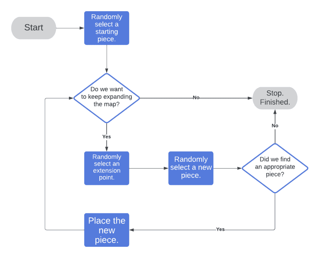
This seems very simple, but what does it look like?

Here we’ve randomly generated a building structure. We started with the entrance hall – which is the only piece placed that has doors opening from the outside. We’ve then repeatedly selected the next place to position something, and the next piece to place, until we’ve got a layout that we’re happy with.
In this example, we’ve shown just simple room outlines. But in practice, the pieces could be fully populated. Instead of laying down just room outlines, we could’ve laid down a kitchen, a sitting room, a conservatory and so on. All of which are fully modelled and ready to use. This would then give a high-quality map that has been randomly generated and will be different for every player.
We’ve just seen how we can generate a totally unique map from pre-existing pieces. However, this still requires those pieces to have been previously created. That, in turn, means an amount of production work needs to be done ahead of time.
What if we want to instead generate a world map? Theoretically, we could do this in a similar manner. However, we can use other techniques to give us a more varied and unique landscape with less production work needed ahead of time.
When generating a 2D world, our main objective is essentially to draw a single line from left to right. This line acts as our ground. Everything above is the sky, and everything below is the land:
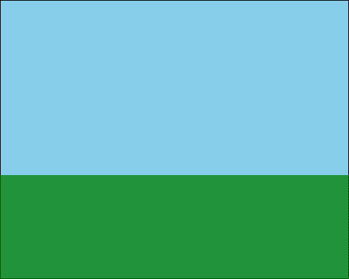
However, this is a pretty boring map. We want something more interesting, so we want to adjust the height of our land across the landscape.
The naive approach to this is to just randomly shift it up or down a little bit for every pixel:
algorithm RandomLandOffsets(landSize, initialHeight, upVariability, downVariability):
    // INPUT
    //    landSize = the size of the land
    //    initialHeight = the initial height of the land
    //    upVariability = the maximum upward height variability
    //    downVariability = the maximum downward height variability
    // OUTPUT
    //    heights = the heights of the land

    heights <- [ ]
    lastHeight <- initialHeight

    for index <- 0 to landSize:
        offset <- random(downVariability, upVariability)
        lastHeight <- lastHeight + offset
        heights[index] <- lastHeight

    return heights
For example, let’s use this to draw a landscape of length 500 pixels, with an initial height of 150 pixels and random variability between -10 and +10 pixels on each step.
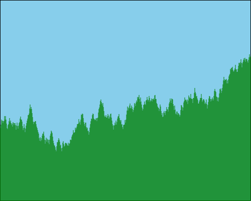
This works. It looks more interesting, but it doesn’t look very realistic. The map is too jagged and spiky. We also have the risk of the landscape running away from us – feasibly, it could just go up or down too far:
One option we have for tackling this is to adjust our offsets based on the distance from the baseline. This will then give us much smoother extremities and will also make it impossible to shift too far from our starting point:
algorithm RestrictedRandomLandOffsets(LandSize, InitialHeight, UpVariability, DownVariability, VariabilityCap):
// INPUT
// LandSize = the size of the land
// InitialHeight = the initial height of the land
// UpVariability = the maximum upward variability
// DownVariability = the maximum downward variability
// VariabilityCap = the cap for variability to limit the distance from the baseline
// OUTPUT
// LandHeights = the heights of the land generated with restricted random offsets
heights <- []
lastHeight <- InitialHeight
for index <- 0 to LandSize:
up <- UpVariability
down <- DownVariability
percentage <- max(1 - abs((lastHeight - InitialHeight) / VariabilityCap), 0)
if lastHeight > InitialHeight:
offset <- random(down, up * percentage)
else:
offset <- random(down * percentage, up)
lastHeight <- lastHeight + offset
heights[index] <- lastHeight
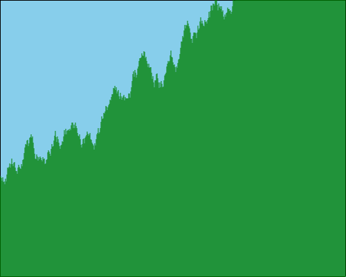
return heightsIf we use this with a variability cap of 200, then we might get something like this:
So we’ve removed any extremes in deviation, but we still have a very jagged appearance.
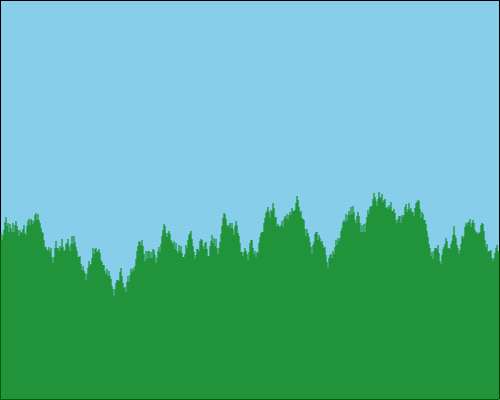
Let’s attempt to sort out this jagged appearance. One way that we can do this is to generate fewer points spread much further apart, and then generate intermediate points between them to generate smooth curves:
algorithm InterpolationBetweenPoints(landSize, initialHeight, up, down, variabilityCap, pointGaps):
    // INPUT
    //    landSize = the size of the land to generate
    //    initialHeight = the initial height of the land
    //    up = the maximum upward variability in height
    //    down = the maximum downward variability in height
    //    variabilityCap = the cap on height variability
    //    pointGaps = the number of pixels between major points
    // OUTPUT
    //    The generated land heights

    majorPoints <- generateHeights((landSize / pointGaps) + 1, initialHeight,
                                    up, down, variabilityCap)
    heights <- [ ]

    for point <- 0 to majorPoints.length - 1:
        left <- majorPoints[point]
        right <- majorPoints[point + 1]
        step <- (right - left) / pointGaps

        for index <- 0 to pointGaps:
            heights[(point * pointGaps) + index] <- left + (step * index)

    return heights
If we do this with a gap between our generated points of 20 pixels – meaning that we have 25 segments – then we might get something like this:
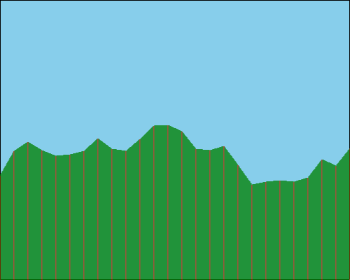
We can immediately see that we have a much smoother appearance. And how this looks can be adjusted by changing how we interpolate between our points. For example, we could choose to draw curves between a set of points instead of just straight lines between adjacent points.
We’ve seen how to generate a realistic-looking 2D map, but what about a 3D map? What we’ve just seen is a simplification of Perlin Noise. This is a technique developed by Ken Perlin in 1983 to generate gradient noise, which gives a random yet realistic-looking pattern of heights.
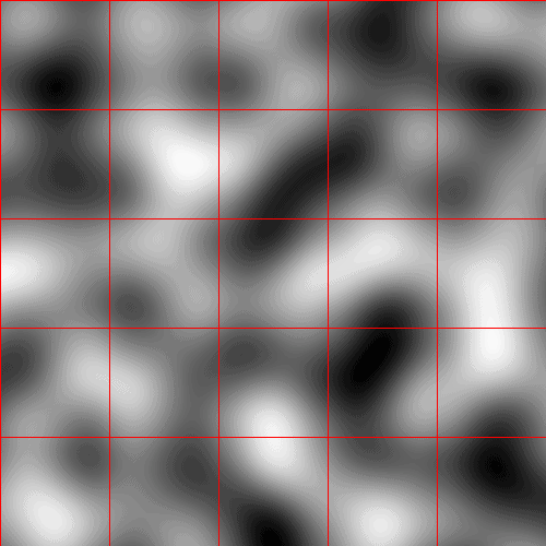
Perlin Noise first generates a coarse grid of random gradient vectors overlaying our map. We can then compute a value for any position in our map such that the transitions between points will always be smooth. This is done by:
This can be done in any number of dimensions, but we’ll work in 2D here. We’ll then treat every point on our 2D perlin noise as the height of the corresponding position in our 3D world:
This will then give us something like this:
This doesn’t look like much, but let’s try colouring it in a bit:
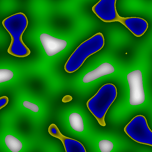
Suddenly, this looks like a realistic map.
So, how does this all work? The overall algorithm for perlin noise is:
algorithm PerlinNoise(landSize, gridSize):
    // INPUT
    //    landSize = dimensions of the land
    //    gridSize = dimensions of the grid
    // OUTPUT
    //    heights = the height values for the land

    grid <- randomGrid(landSize.width / gridSize.width, landSize.height / gridSize.height)

    heights <- []

    for x <- 0 to landSize.width:
        for y <- 0 to landSize.height:
            gridCell <- determineGridCell(gridSize, x, y)
            corners <- getGridCorners(grid, gridCell)
            offsets <- calculateOffsetVectors(gridCell)
            dotProducts <- calculateDotProducts(corners, offsets)
            height <- interpolate(gridCell, dotProducts)
            heights[x, y] <- height

    return heights
The first thing we need to do is generate our random grid. This is a grid of random gradient vectors that overlays the map but is much coarser. The exact way this works isn’t important, but here we’re generating a random angle  and then using trigonometry to calculate the
  and
and  values for our vector.
This has the advantage that we’re only generating a single random number per point and that we’re guaranteed to generate a unit vector:
algorithm PerlinNoiseGenerateRandomGrid(gridSize):
    // INPUT
    //    gridSize = the dimensions of the grid
    // OUTPUT
    //    grid = the generated random grid

    grid <- [ ]

    for x <- 0 to gridSize.width:
        for y <- 0 to gridSize.height:
            theta <- random(0, 2 * π)
            grid[x, y] <- { x: cos(theta), y: sin(theta) }

    return grid
After this, we start calculating values for every map point. From here on, there’s no randomness left. Everything is just calculating some values based on our random gradients and the relative positions on the map to them. This means that we can potentially store the random grid and just compute every map value on demand.
For each point on the map, we first need to determine which cell in our grid we’re in, and where we are within that grid cell. Ultimately this leaves us with two vectors for each corner of the grid cell that we’re in. The first is the random gradient vector for that corner, and the other is a vector from that corner to our position in the cell:
algorithm DetermineGridPositions(gridSize, x, y):
    // INPUT
    //    gridSize = the size of each grid cell
    //    x = the x-coordinate of the point
    //    y = the y-coordinate of the point
    // OUTPUT
    //    gridX, gridY, offsetX, offsetY = the grid cell indices and offsets within the cell

    gridX <- floor(x / gridSize.width)
    gridY <- floor(y / gridSize.height)
    offsetX <- (x / gridSize.width) - gridX
    offsetY <- (y / gridSize.height) - gridY

    return gridX, gridY, offsetX, offsetY

algorithm GetGridCorners(grid, gridCell):
    // INPUT
    //    grid = the grid of random gradient vectors
    //    gridCell = the current grid cell {gridX, gridY, offsetX, offsetY}
    // OUTPUT
    //    tl, tr, bl, br = the gradient vectors at the four corners of the grid cell

    tl <- grid[gridCell.gridX, gridCell.gridY]
    tr <- grid[gridCell.gridX + 1, gridCell.gridY]
    bl <- grid[gridCell.gridX, gridCell.gridY + 1]
    br <- grid[gridCell.gridX + 1, gridCell.gridY + 1]

    return tl, tr, bl, br

algorithm CalculateOffsetVectors(gridCell):
    // INPUT
    //    gridCell = the current grid cell {gridX, gridY, offsetX, offsetY}
    // OUTPUT
    //    tl, tr, bl, br = the offset vectors from the corners of the grid cell to the point

    tl <- {x: gridCell.offsetX, y: gridCell.offsetY}
    tr <- {x: gridCell.offsetX - 1, y: gridCell.offsetY}
    bl <- {x: gridCell.offsetX, y: gridCell.offsetY - 1}
    br <- {x: gridCell.offsetX - 1, y: gridCell.offsetY - 1}

    return tl, tr, bl, br
Having done this, we compute the dot product for each pair of vectors that we have. We then interpolate these dot products together based on the appropriate position within the grid cell that they came from. At the end of this, we have a single value left, which is used as the height for this map position.
def dotProduct(v1, v2):
    // INPUT
    //    v1 = first vector with properties x and y
    //    v2 = second vector with properties x and y
    // OUTPUT
    //    The dot product of v1 and v2

    return (v1.x * v2.x) + (v1.y * v2.y)

def calculateDotProducts(corners, offsets):
    // INPUT
    //    corners = a map with keys tl, tr, bl, br representing the corners of the grid cell and their gradient vectors
    //    offsets = a map with keys tl, tr, bl, br representing the offset vectors from the corners to the point in the grid cell
    // OUTPUT
    //    tl, tr, bl, br = the dot products of each corner and its corresponding offset

    tl <- dotProduct(corners.tl, offsets.tl)
    tr <- dotProduct(corners.tr, offsets.tr)
    bl <- dotProduct(corners.bl, offsets.bl)
    br <- dotProduct(corners.br, offsets.br)

    return {tl, tr, bl, br}

def smoothstep(offset, v1, v2):
    // INPUT
    //    offset = the offset within the grid cell
    //    v1 = the value at the starting point
    //    v2 = the value at the ending point
    // OUTPUT
    //    the interpolated value between v1 and v2

        fade <- (6 * offset^5) - (15 * offset^4) + (10 * offset^3)

        return v1 + (fade * (v2 - v1))

def interpolate(gridCell, dotProducts):
    // INPUT
    //    gridCell = a map with properties offsetX and offsetY
    //    dotProducts = a map with keys tl, tr, bl, br representing the dot products for the corners
    // OUTPUT
    //    The interpolated height value for the point inside the grid cell

    t <- smoothstep(gridCell.offsetX, dotProducts.tl, dotProducts.tr)
    b <- smoothstep(gridCell.offsetX, dotProducts.bl, dotProducts.br)

    return smoothstep(gridCell.offsetY, t, b)
This uses the Smoothstep function for interpolation since this gives a smoother transition between cells. However, we can use any interpolation function that we want to combine our values.
This seems complicated, so let’s work through it for real. Specifically, we’ll work out the values for this map position:
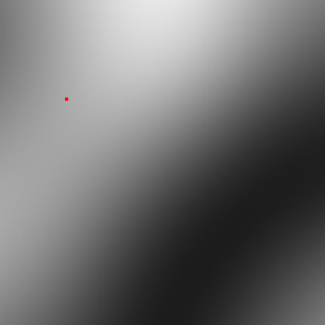
This is position  in our overall map. We have a grid of size
  overlaying our map, so our grid cell for this looks:
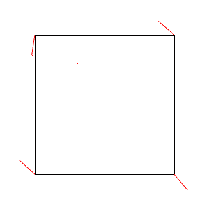
For this cell, our random vectors on the corners are:


And our offset vectors are:


From these, we can compute our dot products:


Finally, we interpolate these values together for our final value:


So we have calculated a height value for this map point of 0.1873.
If we follow this process for every single map point, we’ll have generated our height map. We can then normalize these – by finding the highest and lowest values calculated and scaling every point based on those – so that we can understand what the map really looks like. For example, on our above map, the lowest calculated value was  and the highest calculated value was
  . This means that this exact point normalises to
  in a range of
  to
to  .
.
Our above coloured-in map was done by treating everything with a value below  as water, below
  as sand, below
  as grass and everything above as mountainous. So, means it’s on the higher end of grassland.
Here we’ve seen some techniques for the procedural generation of maps. A huge variety of such techniques and many more variations are within them. Further, we can mix and match as appropriate.
For example, we could use perlin noise to generate a landscape and then populate it with buildings generated using random piece allocation. Why not try this out for yourself and see how it goes?