Finding the Number of Occurrences of a Subsequence in a String

1. Overview

In this tutorial, we’ll discuss the problem of finding the number of occurrences of a subsequence in a string. First, we’ll define the problem. Then we’ll give an example to explain it. Finally, we’ll present three different approaches to solve this problem.

2. Defining the Problem

We have a string $S$ and a string $T$ . We want to count the number of times that string $T$ occurs in string $S$ as a subsequence.

A subsequence of a string is a sequence that can be derived from the given string by deleting zero or more elements without changing the order of the remaining elements.

Let’s take a look at the following example for a better understanding.

Given a string $S = "ababc"$ and a string $T = "abc"$ :

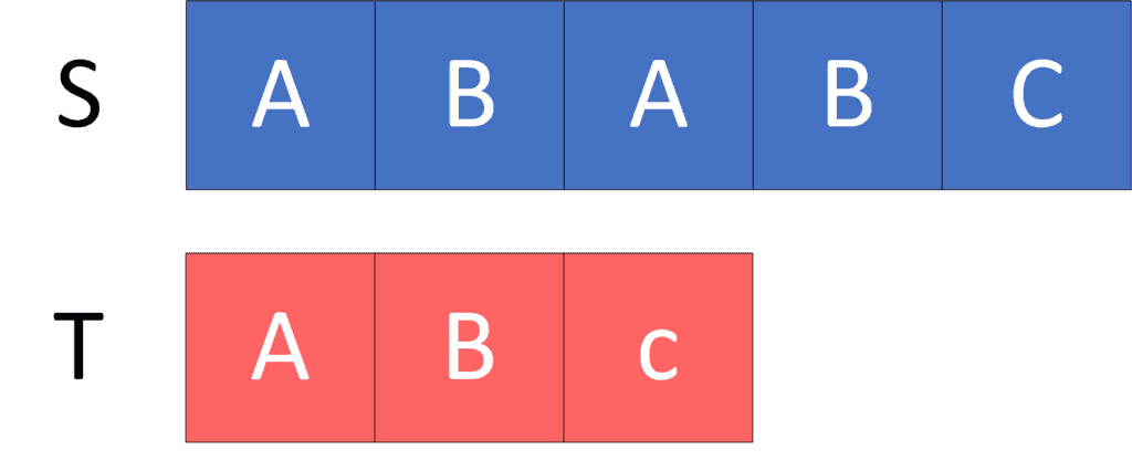
Let’s count the number of occurrences of string $T$ in string $S$ as a subsequence:

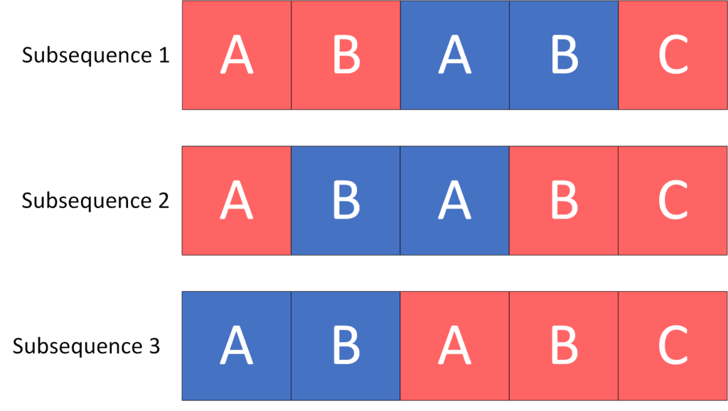
As we can see, there are three subsequences of string $S$ that are equal to the string $T$ . Thus, the answer to the given example is $3$ .

3. Recursion Approach

The main idea in this approach is to try every possible subsequence of the string $\mathbf{S}$ and see if it matches the string $\mathbf{T}$ .

For each character of the string $S$ , we’ll have two options. We can leave it so that we don’t consider it in the current subsequence, and we move to the next character. Otherwise, we can take it as a character in our subsequence if it’s equal to the current character of the string $T$ .

When we reach the end of the string $T$ , we get a subsequence of the string $S$ that’s equal to the string $T$ . As a result, we increase the count of the subsequences by one. Otherwise, we ignore the current subsequence.

3.1. Algorithm

Let’s take a look at the implementation of the algorithm:

Initially, we declare the $countOccurences$ function that will return the number of subsequences of the string $S$ that match the string $T$ . The function will have two parameters, $i$ and $j$ , which will represent our current position in the string $S$ and $T$ , respectively.

First, since we’re dealing with a recursive function, we’ll set the base conditions to stop searching for answers. We have two situations we have to handle:

If we reach the end of $S$ and $T$ , that means we got a subsequence of $S$ that matches the string $T$ , so we return $1$ to increase the number of subsequences.
If we reach the end of the string $S$ , that means we didn’t reach the end of $T$ . Therefore, we didn’t find a subsequence that matches $T$ , and we return $0$ .

Second, we have to set the recursive calls. For each character of $\mathbf{S}$ , we have two options; we can either pick the current character, or leave it:

Pick: if the current character of $S$ matches the current character of $T$ , we try to take it and move both pointers forward.
Leave: for each character of $S$ , we also have to consider it out of our subsequence. Thus, we try to leave it and move only the pointer of $S$ forward.

The sum of these two recursive calls will eventually be the answer to the current state.

Finally, the $countOccurences(0, 0)$ will return the number of subsequences of the string $S$ that match the string $T$ .

3.2. Complexity

The time complexity of this algorithm is $\mathbf{O(2^{min(N, M)})}$ , where $N$ is the length of the string $S$ , and $M$ is the length of string $T$ . The reason for this complexity is that for each character of the string $S$ , we have two choices, whether we take it or leave it. However, the picking step is limited to the number of characters inside $T$ . So, that gives us a total complexity of $O(2^{min(N, M)})$ .

The space complexity of this algorithm is $\mathbf{O(N)}$ , since the depth of the recursion tree will be at most $N$ , as each time we move to the next character in the string $S$ .

4. Dynamic Programming Approach

The huge complexity of the previous approach comes from calculating each state $(i, j)$ multiple times. In this approach, we’ll try to memorize the answer of each state $\mathbf{(i, j)}$ to use it in the future without calculating that state again.

As we see in the previous approach, the answer of state $(i, j)$ depends on the answers of the state $(i + 1, j + 1)$ , and the state $(i + 1, j)$ . Therefore, we’ll calculate $(i + 1, j + 1)$ and $(i + 1, j)$ before calculating the state $(i, j)$ . Then we’ll calculate the answer of the state $(i, j)$ depending on the previous answers.

Finally, the answer to our problem will be stored in the answer of the state $(0, 0)$ .

4.1. Algorithm

Let’s take a look at the implementation of the algorithm:

Initially, we declare the $DP$ array, which will store the answer of each state $(i, j)$ . The initial value of the state $(length(s), length(T))$ is equal to $1$ , since this was the base case in the previous approach.

Next, we’ll iterate from the end of the string $S$ until the beginning. For each position in the string $S$ , we’ll also iterate over the string $T$ from the end until the beginning because every state is depending on the states that come after it.

For each state $(i, j)$ , we’ll check if the current characters of both strings match. If so, we’ll add to the answer of the current state the answer of state $(i + 1, j + 1)$ , which means we picked the current character of the string $S$ . In addition, we add the answer of the state $(i + 1, j)$ , which means we leave the current character of the string $S$ .

Finally, the value of $DP[0][0]$ is equal to the number of subsequences of the string $S$ that match the string $T$ if we start from the beginning of both strings.

4.2. Complexity

The complexity of this algorithm is $\mathbf{O(N \times M)}$ , where $N$ is the length of the string $S$ , and $M$ is the length of the string $T$ . The reason for this complexity is that for each character of the string $S$ , we iterate over all the characters of the string $T$ , and try to solve each state individually depending on the states that we calculated earlier.

The space complexity of this algorithm is $\mathbf{O(N \times M)}$ , which is the size of the memoization array that we use to store the answer of each state.

5. Dynamic Programming Optimization

In this approach, we’ll optimize the space complexity of the previous one. The main idea here will be the same as the previous approach. The only difference is that since each state $\mathbf{(i, j)}$ depends only on the next state $\mathbf{(i + 1, x)}$ , where $\mathbf{0 \le x < length(T)}$ represents any position of the string $\mathbf{T}$ , we can reduce the first dimension of the memoization array to $\mathbf{2}$ instead of $\mathbf{N}$ (the length of the string $\mathbf{S}$ ).

For each state, we’ll try to store it in an alternating position of the next state. To do that, we’ll get the advantage of the mod operator. So, $i \bmod 2$ will be the current state, and $1 - i \bmod 2$ or $(i + 1) \bmod 2$ will be the next state.

In the end, the answer to our problem will also be stored in the answer of the state $(0, 0)$ .

5.1. Algorithm

Let’s take a look at the implementation of the algorithm:

Initially, we declare the $DP$ array, which will store the answer of each state $(i, j)$ . The initial value of the state $(length(S) \bmod 2, length(T))$ is equal to $1$ , since it’s the base case here.

Next, we’ll do the same as the previous approach, but instead of putting the original index in the first dimension, we’ll put its module by $2$ .

Finally, the value of $DP[0][0]$ is equal to the number of subsequences of the string $S$ that match the string $T$ if we start from the beginning of both strings.

5.2. Complexity

The space complexity of this algorithm is $\mathbf{O(2 \times M)}$ , which is the size of the memoization array that we use to store the answer of each state. The first dimension becomes equal to $2$ , since the answer of each position $i$ in the string $S$ depends only on the answer of the next position, $i + 1$ .

6. Conclusion

In this article, we presented the problem of finding the number of occurrences of a subsequence in a string.

First, we provided an example to explain the problem. Then we explored three different approaches for solving it.

Finally, we walked through their implementations, with each approach having a better space or time complexity than the previous one.

Full Archive

About Baeldung

Core Concepts

Operating Systems

Artificial Intelligence

Graph Theory

Latex

1. Overview

2. Defining the Problem

3. Recursion Approach

3.1. Algorithm

3.2. Complexity

4. Dynamic Programming Approach

4.1. Algorithm

4.2. Complexity

5. Dynamic Programming Optimization

5.1. Algorithm

5.2. Complexity

6. Conclusion