

Learn through the super-clean Baeldung Pro experience:
>> Membership and Baeldung Pro.
No ads, dark-mode and 6 months free of IntelliJ Idea Ultimate to start with.
Learn through the super-clean Baeldung Pro experience:
>> Membership and Baeldung Pro.
No ads, dark-mode and 6 months free of IntelliJ Idea Ultimate to start with.
In this tutorial, we’ll explain the extended Euclidean algorithm (EEA). It’s a tool widely used in cryptography and one of the fundamental algorithms in number theory. In addition to its recursive version, we’ll present its iterative variant.
Bézout’s identity states that the greatest common divisor (GCD) of any two integers is their linear combination. So, if  is the GCD of
  and
and  , then there exist integers
  and
and  such that:
(1) 
For example, if  and
and  , then
  and:
and:
![\[1 = -1\cdot 5 + 2\cdot 3\]](/wp-content/ql-cache/quicklatex.com-aac1d9b162c5c4a050d7ab0304d48bf1_l3.svg "Rendered by QuickLaTeX.com")
The extended Euclidean algorithm (EEA) finds  and
and  , which are called Bézout’s coefficients of
  and
and  . As we’ll see, EEA is a modification of the Euclidean algorithm for finding the GCD of two numbers.
In what follows, we’ll assume that and are both positive and that  . We lose no generality under those assumptions because:
![\[\begin{aligned} GCD(a, b) &=&& GCD(|a|, |b|) \\ GCD(a, b) &=&& GCD(b, a) \\ GCD(a, 0) &=&& a \end{aligned}\]](/wp-content/ql-cache/quicklatex.com-69a8bceccd0a45deb02c68bdbdcdd8bd_l3.svg "Rendered by QuickLaTeX.com")
which means that we can consider only the case  :
:
and is zero, then we output the other number as their GCD and set the corresponding coefficients to  and
and  . (or ) is negative, then we replace it with its absolute value. and if
  .
.The Euclidean algorithm (EA) finds the GCD of and by using the fact that:
![\[GCD(a, b) = GCD(b, a\bmod b)\]](/wp-content/ql-cache/quicklatex.com-29b46bf4bfddc5446fffdefdd9e2591b_l3.svg "Rendered by QuickLaTeX.com")
and applying Euclidean division until it gets zero as the remainder:
![\[\begin{aligned} \underbrace{a}_{a_1} &=&& \underbrace{\left\lfloor\frac a b \right\rfloor}_{q_1}\cdot \underbrace{b}_{a_2} + \underbrace{(a \bmod b)}_{a_3} &&(1\leq a_3 < b)\\ a_2 &=&& q_2\ a_3 + a_4 &&(1 \leq a_4 < a_3)\\ \vdots \\ a_{n-3} &=&& q_{n-3} a_{n-2} +a_{n-1} && (1 \leq a_{n-1} < a_{n-2}) \\ a_{n-2} &=&& q_{n-2} a_{n-1} +a_{n} && (1 \leq a_{n} < a_{n-1}) \\ a_{n-1} &=&& q_{n-1} a_{n} +a_{n+1} && (1 \leq a_{n+1} < a_n) \\ a_{n} &=&& q_{n}a_{n+1} + 0 &&(a_{n+2}=0) \end{aligned}\]](/wp-content/ql-cache/quicklatex.com-ccbf003366056d464c39869a9a6873e3_l3.svg "Rendered by QuickLaTeX.com")
The last nonzero remainder ( ) is the GCD of and . As we see, the recursion is:
(2) 
where  . We’ll find it useful to re-formulate the recursive rule so that we express the remainder in terms of the dividend and the divisor:
(3) 
The recursive extension of EA (REEA) runs just like the regular EA until it computes  , the GCD of the input numbers and . At that point, it starts recursing back to the beginning, revisiting the division steps of
  backward. After backtracking to a division step, REEA expresses the GCD as a combination of the step’s divisor and dividend.
So, from the second-to-last division, we get:
![\[a_{n+1} = a_{n-1} -q_{n-1}a_{n} \\\]](/wp-content/ql-cache/quicklatex.com-f69def49f440a337d2a9f62b81099cff_l3.svg "Rendered by QuickLaTeX.com")
Now, backtracking to  , we replace
  with
with  , so we have:
![\[\begin{aligned} a_{n+1} &=&& a_{n-1} - q_{n-1}(a_{n-2}-q_{n-2}a_{n-1}) \\ &=&& (1+q_{n-1}q_{n-2})a_{n-1} +(- q_{n-1})a_{n-2} \end{aligned}\]](/wp-content/ql-cache/quicklatex.com-5e84e0fd336c0a7f58a427f34278b2ea_l3.svg "Rendered by QuickLaTeX.com")
In general, let’s say we revisited the division step  and expressed
  as a linear combination of
  and
and  :
:
(4) 
Recursing one step back, we substitute with  in Equation (4):
(5) 
Therefore, we obtain the following backward recursive rules:
(6) 
We apply them going backward through the division steps until we finally represent the GCD as a linear combination of  and
and  :
:
algorithm RecursiveExtendedEuclideanAlgorithm(a, b):
    // INPUT
    //    a, b = two non-negative integers
    // OUTPUT
    //    d = the greatest common divisor (GCD) of a and b
    //    x, y = integers such that d = x * a + y * b

    if b = 0:
        d <- a
        x <- 1
        y <- 0

        return (d, x, y)

    q <- floor(a / b)
    r <- a mod b
    (d, x, y) <- RecursiveExtendedEuclideanAlgorithm(b, r)

return (d, y, x - q * y)Let’s say that  and
and  . Applying the algorithm, we do five Euclidean divisions:
![\[\begin{aligned} 254 &= 5\cdot 44 + 34 \\ 44 &= 1\cdot 34 + 10 \\ 34 &= 3\cdot 10 + 4 \\ 10 &= 2\cdot 4 + \boldsymbol{2}\\ 4 &= 2\cdot 2 + 0 \end{aligned}\]](/wp-content/ql-cache/quicklatex.com-801be2d7d7e26afd228bd9c01506f0d8_l3.svg "Rendered by QuickLaTeX.com")
Or, using recurrence (3):
![\[\begin{aligned} 34 &= 254 - 5\cdot 44 \\ 10 &= 44 - 1 \cdot 34 \\ 4 &= 34 - 3 \cdot 10 \\ \boldsymbol{2} & = 10 - 2\cdot 4 \\ 0 &= 4 - 2\cdot 2 \end{aligned}\]](/wp-content/ql-cache/quicklatex.com-d13a07d9f011827150ec7beb7ea3cbc7_l3.svg "Rendered by QuickLaTeX.com")
After identifying the GCD, we go backward one division step. From there, we get  and climb one step up to see what to substitute
  with:
with:
![\[\begin{aligned} &\downarrow && 34 = 254 - 5\cdot 44 && & \\ &\downarrow && 10 = 44 - 1 \cdot 34 && & \\ &\downarrow && 4 = 34 - 3 \cdot 10 && 2 = 1\cdot 10 + (-2)\cdot (34 - 3\cdot 10) & \\ &\downarrow && 2 = 10 - 2\cdot4 && 2 = 1\cdot 10 + (-2)\cdot 4 & \uparrow \\ & && 0 = 4 - 2\times 2 && & \uparrow \\ \end{aligned}\]](/wp-content/ql-cache/quicklatex.com-7887a3527c28f7a7d808895b71fc285a_l3.svg "Rendered by QuickLaTeX.com")
After some elementary algebra, we get that  . Then, we go up a step again to see what to replace
  with:
with:
![\[\begin{aligned} &\downarrow && 34 = 254 - 5\cdot 44 && & \\ &\downarrow && 10 = 44 - 1 \cdot 34 && 2 = (-2)\cdot 34 + 7\cdot(44 - 1\cdot 34)& \\ &\downarrow && 4 = 34 - 3 \cdot 10 && 2 = (-2)\cdot 34 + 7\cdot 10 & \uparrow\\ &\downarrow && 2 = 10 - 2\cdot4 && 2 = 1\cdot 10 + (-2)\cdot 4 & \uparrow\\ & && 0 = 4 - 2\times 2 && & \uparrow \end{aligned}\]](/wp-content/ql-cache/quicklatex.com-82f90d18885948c5e6140e7fe759e9e8_l3.svg "Rendered by QuickLaTeX.com")
and get  . In the end, we backtrack to the first division step:
![\[\begin{aligned} &\downarrow && 34 = 254 - 5\cdot 44 && 2 = 7\cdot 44 - 9\cdot(254-5\cdot 44)& \\ &\downarrow && 10 = 44 - 1 \cdot 34 && 2 = 7\cdot 44 + (-9)\cdot 34 & \uparrow \\ &\downarrow && 4 = 34 - 3 \cdot 10 && $2 = (-2)\cdot 34 + 7\cdot 10 & \uparrow\\ &\downarrow && 2 = 10 - 2\cdot4 && 2 = 1\cdot 10 + (-2)\cdot 4 & \uparrow \\ &&& 0 = 4 - 2\times 2 && & \uparrow \end{aligned}\]](/wp-content/ql-cache/quicklatex.com-7cb60ef5c33ea4363f95f8461be2683c_l3.svg "Rendered by QuickLaTeX.com")
and obtain Bézout’s coefficients:
(7) 
We can compute the coefficients without backtracking. The idea is to express each step’s remainder as a linear combination of and . To do so, we start by noting that:
![\[\begin{aligned} a_1 &=&& \underbrace{1}_{x_1}\cdot a_1 + \underbrace{0}_{y_1} \cdot a_2 \\ a_2 &=&& \underbrace{0}_{x_2}\cdot a_1 + \underbrace{1}_{y_2} \cdot a_2 \end{aligned}\]](/wp-content/ql-cache/quicklatex.com-358ea5c264d038eb4891b6ab18dd8258_l3.svg "Rendered by QuickLaTeX.com")
In general, we’ll have:
(8) 
and we want rules for calculating the coefficients in a step given those from the previous steps. As it turns out, we need only the coefficients from the previous two steps. So, let’s suppose that we know  ,
,  ,
,  , and
, and  for some
  :
:
![\[\begin{aligned} a_{k} &=&& x_ka_1+y_ka_2 \\ a_{k+1} &=&& x_{k+1}a_1+y_{k+1}a_2 \end{aligned}\]](/wp-content/ql-cache/quicklatex.com-ef8f6776431b633f472e77eaba22f488_l3.svg "Rendered by QuickLaTeX.com")
Using Equation (3), we get:
(9) 
Hence, these are our forward recurrences for the coefficients:
(10) 
We start from  and
and  and gradually work our way through division steps until we calculate the GCD, at which point we also obtain the sought Bézout’s coefficients:
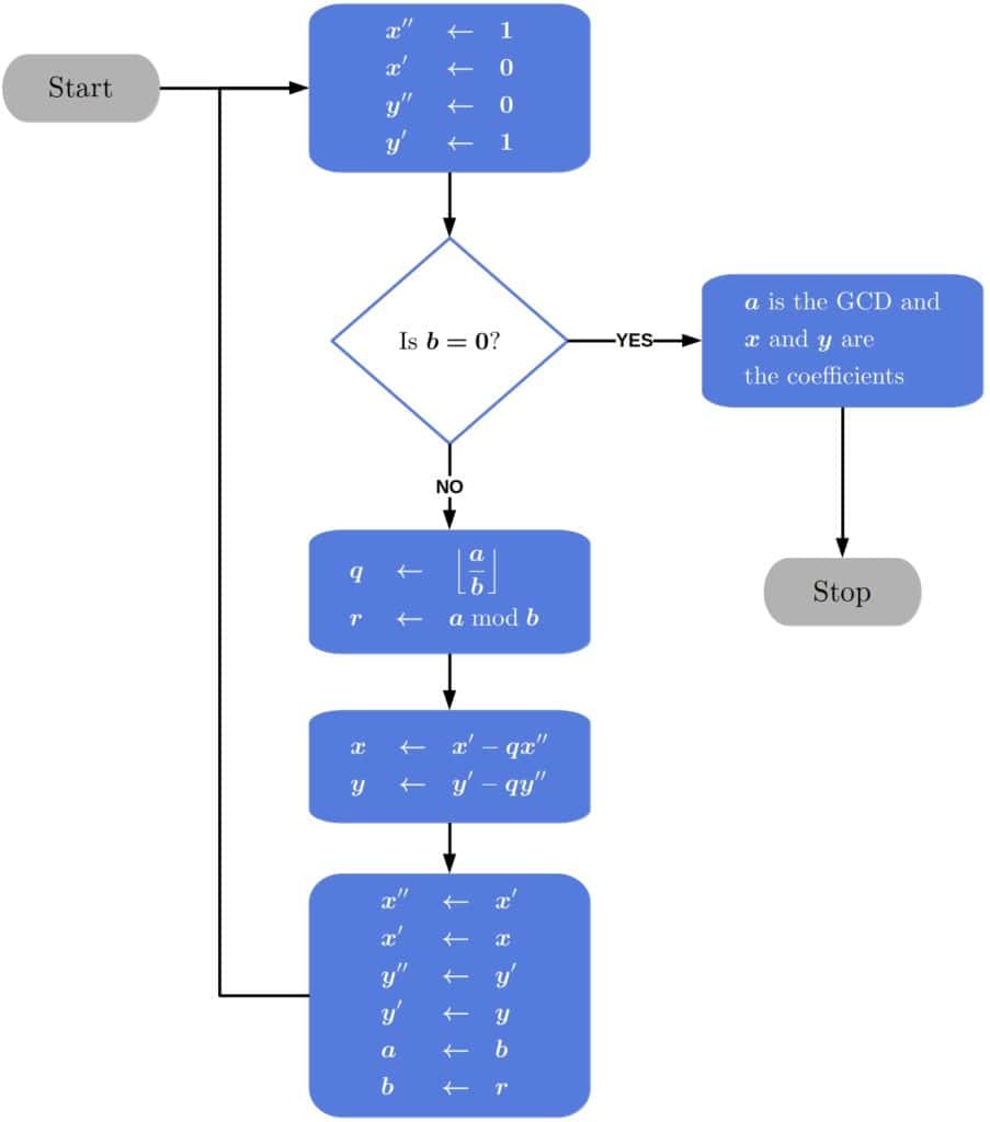
algorithm terativeExendedEuclideanlgorithm(a, ):
    // INUT
    //   a, b = two positive integers
    // OUTPUT
    //    d = the GCD of a and b
    //    x, y = the coefficients such that d = GCD(a, b) and d = xa + yb
    //    x``, x`, y``, and y` correspond to x_k, x_{k+1}, y_k, y_{k+1} in recurrences (10)

    x`` <- 1
    x`  <- 0
    y`` <- 0
    y`  <- 1

    while b > 0:
        q <- a div b
        r <- a mod b

        x <- x` - q * x``
        y <- y` - q * y``

        x`` <- x`
        x` <- x
        y`` <- y`
        y` <- y

        a <- b
        b <- r

    d <- a

    return (d, x, y)
This is how it’ll look like step by step:
This iterative form of the EEA is equivalent to the Blankinship method for two numbers, which extends EA to find the GCD and Bézout’s coefficients of  numbers, not just two.
Let’s reuse the example for REEA. Here, we compute the coefficients as we perform Euclidean divisions. The first remainder,  , is a direct linear combination of
  and
and  :
:
![\[254 = 5\cdot 44 + 34 \implies 34 = 1\cdot 254 + (-5)\cdot 44 \\\]](/wp-content/ql-cache/quicklatex.com-a0dd6a4e0db3f7725abf1ad3562713a0_l3.svg "Rendered by QuickLaTeX.com")
Next, we divide with . Then, we express the remainder as a linear combination of and and replace with the expression we got in the previous step:
![\[\begin{aligned} &\downarrow & 254 &=& 5\cdot 44 + 34 && 34 &=&& 1\cdot 254 + (-5)\cdot 44\\ & & 44 &=& 1\cdot 34 + 10 && 10 &=&& 44 - 1\cdot 34\\ & & && && 10 &=&& 44-1(254-5\cdot 44)\\ & & && && 10 &=&& (-1)\cdot 254+6\cdot 44 \\ \end{aligned}\]](/wp-content/ql-cache/quicklatex.com-ba8ea9bd07081a368ebbd878a9955d33_l3.svg "Rendered by QuickLaTeX.com")
We obtain the coefficients by repeating the step. After each division step, we express the remainder in terms of the current dividend and the divisor. Since both have appeared as remainders previously, we replace them with the corresponding linear combinations and simplify the expressions:
![\[\begin{aligned} &\downarrow & 254 &=& 5\cdot 44 + 34 && 34 &= 1\cdot 254 + (-5)\cdot 44\\ &\downarrow & 44 &=& 1\cdot 34 + 10 && 10 &=(-1)\cdot 254+6\cdot 44 \\ &\downarrow & 34 &=& 3\cdot 10 + 4 && 4 &=34 - 3\cdot 10\\ &&&&&&4&=(1\cdot 254 - 5\cdot 44)-3(-254+6\cdot 44)\\ &&&&&&4&=4\cdot 254+(-23)\cdot 44\\ &&10 &=& 2\cdot 4 + 2 && 2 &= 1\cdot 10 + (-2)\cdot 4\\ &&&&&&2&= 1\cdot(-254+6\cdot 44)-2\cdot (4\cdot 254-23\cdot 44)\\ &&&&&&2&= (-9)\cdot 254 + 52\cdot 44 \end{aligned}\]](/wp-content/ql-cache/quicklatex.com-1d9d2d42c1387d26b34f91623c9a873c_l3.svg "Rendered by QuickLaTeX.com")
We get the same result as with REEA in the end, but without recursion. Generally, the iterative variant should be faster because it avoids recursive calls and keeps the same frame.
As we see from the recurrences (10), the -coefficients and -coefficients don’t depend on one another. Moreover, from the final form:
![\[GCD(a, b) = x\cdot a + y \cdot b\]](/wp-content/ql-cache/quicklatex.com-d59f3ede7c26a21fff6920f27dbc1208_l3.svg "Rendered by QuickLaTeX.com")
we can calculate the final if we know the final :
![\[y = \frac{GCD(a,b)-x\cdot a}{b}\]](/wp-content/ql-cache/quicklatex.com-4353705587904c4dd067619545ef419f_l3.svg "Rendered by QuickLaTeX.com")
and the other way around. So, there’s no need to compute both coefficients as we make division steps. That cuts the number of operations by a third.
Bézout’s coefficients are not unique, In fact, if  is one pair of Bézout’s coefficients for and , then all the coefficients are of the form:
(11) 
where  .
.
Only two pairs satisfy:
(12) 
and EEA always finds one such pair.
In this article, we presented the recursive and iterative forms of the Extended Euclidean Algorithm. It’s used for finding Bézout’s coefficients of two integer numbers and has applications in cryptography.