Network Flow: Dinic’s Algorithm | Baeldung on Computer Science

1. Overview

Dinic’s Algorithm is a powerful tool in computer science for solving network flow problems efficiently. In this tutorial, we’ll take a look at what this algorithm means and what it does.

Then, we’ll go through the steps of the Dinic algorithm. In addition to an example of resolving the maximum flow problem using Dinic’s algorithm, we’ll discuss the time complexity and the use cases of this algorithm.

2. What Is Dinic’s Algorithm

Dinic’s algorithm is a popular algorithm for determining the maximum flow in a flow network. Which is regarded as one of the most effective algorithms for resolving the maximum flow problem. It was created in 1970 by computer scientist Yefim (Chaim) Dinic.

Dinic’s algorithm, which is based on level graphs and blocking flows, has an ${\boldsymbol{O(VE^2)}}$ complexity, where ${\boldsymbol{V}}$ is the number of network vertices (also known as nodes) and ${\boldsymbol{E}}$ is the number of network edges.

Here are additional concepts used in the Dinic algorithm:

Flow network: A flow network is a directed graph in which each edge has a capacity or the most flow that can possibly pass through it. The number of resources actually passing through the edges is represented by the flow in the network.
Source and sink: In a flow network, a source vertex is a special vertex that produces the flow, and a sink vertex is a special vertex that consumes the flow.
Residual graph: The capacity of the edges in the residual graph is updated in accordance with the current flow, making it a modified version of the original flow network. It represents the amount of additional flow that each edge can still handle.
Augmenting path: In the residual graph, an augmenting path is one that connects the source and sink while having positive edge capacities. The network’s flow increases by using augmenting paths.

3. The Analogy to Understand Dinic’s Algorithm

Let’s imagine that this weekend we have plans to visit an amusement park. However, all we know is that it’s 10 minutes south of our house. Since we have never been to this amusement park, we are unsure of its exact location. How do we plan to get there? South, southeast, or southwest are the only directions that make sense to take. This algorithm will make sure that we only move forward in the direction of our goal.

Therefore, the question is how to use this to address the maximum flow issue. The algorithm can be outlined as follows:

Let’s start at the source node and move in the direction of the goal (amusement park) by choosing the edge with the highest residual capacity in the south, southeast, or southwest direction. This ensures that we are always moving towards the goal.
Once we reach a node with no outgoing edges in the south, southeast, or southwest direction, we mark it as the end of the path and backtrack to the previous node.
At each step, we choose the edge with the highest residual capacity in the reverse direction of our previous move (i.e., north, northwest, or northeast) to backtrack.
Then we’ll update the residual capacities of the edges along the path by subtracting the flow from the chosen edge (if any) and adding it to the reverse direction edge.
We’ll repeat steps $\text{1 - 4}$ until we reach the goal (amusement park) or we are unable to find any more augmenting paths.
The maximum flow in the network will be the sum of the flows along all the augmenting paths.

4. Steps for the Dinic’s Algorithm

Let’s now discover how the fundamental components of Dinic’s algorithm interact to produce such an effective algorithm.

4.1. Create the Level Graph

First, we initialize the flow by giving the network a zero initial flow. Then, we create the level graph:

Create the level graph by performing a Breadth-First Search (BFS) from the source vertex, which assigns each vertex a level (or distance) based on how many edges lead to the source
Finding the shortest paths for augmenting is made easier by this step

4.2. Locate Blocking Flows

Let’s now locate blocking flows:

We apply a depth-first search (DFS) to the residual graph to find augmenting paths while taking into account the levels assigned in step ${2}$
If all of the edges along a path have positive capacities, the path is said to be augmenting
The blocking flows that can be used to increase network flow are represented by these augmenting paths. A flow is a Blocking Flow if no more flows can be sent using the level graph

4.3. Update the Flow

By enhancing the flow along the augmenting paths identified in step ${3}$ , we update the network’s flow. This is accomplished by selecting the edge along the augmenting path with the lowest capacity, and adding it to the flow.

Let’s now repeat steps $\text{2 and 4}$ until no additional augmenting paths are visible in the residual graph. The algorithm concludes at this point, and the obtained flow represents the maximum possible flow through the network.

5. Steps for the Dinic’s Algorithm

Here’s an initial residual graph:

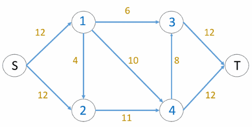
In the initial graph, the $\text{total flow = 0}$ .

5.1. First Iteration

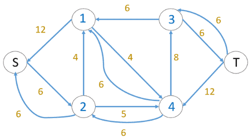
Let’s use BFS to assign levels to all nodes. Then, we investigate whether an additional flow is possible (or there is a $\text{s - t}$ path in the residual graph):

The edges marked with a block sign cannot be used to send flow because they do not connect nodes of a lower level to nodes of a higher level. The blocking flow is found using levels, where every flow path should have levels as 0, 1, 2, 3. Three flows are sent at once, unlike Edmond Karp where only one flow is sent at a time:

6 units of flow are sent on path $\text{S - 1 - 3 - T}$
6 units of flow are sent on path $\text{S - 1 - 4 - T}$
6 units of flow are sent on path $\text{S - 2 - 4 - T}$

The total flow is calculated as $\text{total flow + 6 + 6 + 6 = 18}$ . Then, the residual graph changes to the following after the first iteration:

Residual graph after first iteration of Dinic's algorithm

5.2. Second Iteration

Using the BFS for the above modified residual graph, we assign new levels to all nodes. We also investigate whether an additional flow is possible (or there is a $\text{s - t}$ path in the residual graph):

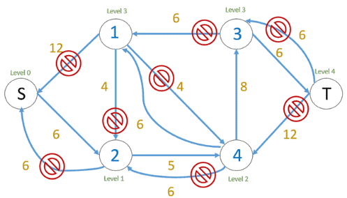
The edges marked with a block sign cannot be used to send flow because they do not connect nodes of a lower level to nodes of a higher level (from level ${i}$ to level ${i + 1}$ ). So, the blocking flow is identified using levels, where every flow path should have levels as 0, 1, 2, 3, 4. In this case, only one flow can be sent at a time:

6 units of flow are sent on path $\text{S - 2 - 4 - 3 - T}$
Total flow is calculated as $\text{Total flow + 5 = 23}$

The residual graph changes to the following after the second iteration:

5.3. Third Iteration

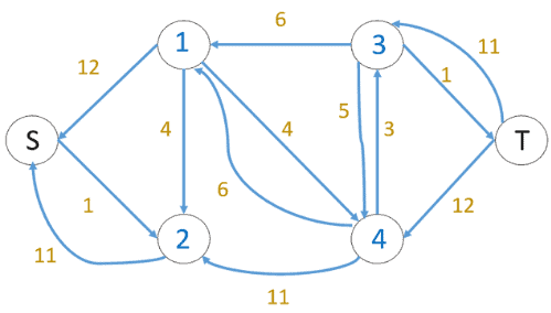
In the third iteration, we run BFS and draw a level graph. We also determine whether more flow is possible and proceed only if it is. There is no $\text{s - t}$ path in the residual graph this time, which means the algorithm is terminated.

6. Implementation of Dinic’s Algorithm

Let’s now look at the implementation of Dinic’s algorithm. Here’s a pseudocode for implementing the algorithm:

Dinic’s algorithm efficiently computes the maximum flow in a flow network. It uses the original flow network ${G}$ and its residual graph ${Gf}$ , with ${s}$ as the source vertex and ${t}$ as the sink vertex.

The algorithm employs ${BFS}$ and ${DFS}$ techniques, utilizing the ${level}$ and ${ptr}$ arrays. In ${Gf}$ , ${neighbors[u]}$ represents the neighbors of vertex ${u}$ .

The algorithm iterates until there are no more augmenting paths in ${Gf.}$ It constructs the level graph using ${BFS}$ and finds augmenting paths using ${DFS}$ to update the network flow ( ${INF}$ is a large constant used as the starting point for bottleneck capacity).

7. Dinic Algorithm Complexity

The algorithm’s complexity is ${O(VE^2)}$ :

First, it takes ${O(E)}$ time to perform a ${BFS}$ to construct a level graph
Then, the time taken to send multiple more flows until a blocking flow is reached is ${O(VE)}$
Finally, it takes ${O(V)}$ to run the outer loop. As a result, the overall time complexity is ${O(VE^2)}$

8. Use Cases for the Dinic Algorithm

Dinic’s algorithm is a powerful algorithm for efficiently solving network flow problems. Here are some examples of appropriate applications for Dinic’s algorithm:

Transportation Networks: Dinic’s algorithm can be used to optimize transportation networks, such as road networks or airline routes. It can be used to optimize the flow of goods from one warehouse to another or to schedule flights in an airline network to minimize costs
Communication Networks: Dinic’s algorithm can be used to optimize the flow of data packets in communication networks, such as routing algorithms for packet-switched networks
Social Networks: Dinic’s algorithm can be used to model social networks, such as online social media networks or transportation networks within cities, in order to study information diffusion, influence propagation, or congestion patterns. It can aid in the optimization of the flow of information, resources, or people within a social network

9. Conclusion

In this tutorial, we provided an overview of Dinic’s algorithm, its steps, implementation, complexity, and use cases. We also highlighted its efficiency in solving network flow problems across diverse domains.

Dinic’s algorithm emerges as a valuable tool for optimizing resources, information, and energy flow in various applications, making it a preferred choice in network flow optimization.

Full Archive

About Baeldung

Core Concepts

Operating Systems

Artificial Intelligence

Graph Theory

Latex