

Learn through the super-clean Baeldung Pro experience:
>> Membership and Baeldung Pro.
No ads, dark-mode and 6 months free of IntelliJ Idea Ultimate to start with.
Learn through the super-clean Baeldung Pro experience:
>> Membership and Baeldung Pro.
No ads, dark-mode and 6 months free of IntelliJ Idea Ultimate to start with.
One of the most simple party games we can play with friends is “Guess Who?”. Each player receives a piece of paper with the name of someone famous and places it on their forehead without reading it.
After that, we should try to guess our character by making questions that can only be answered with yes or no. Some variations might include objects and a specific score counting system.
We can also play this game in a more modern way by using mobile apps or websites.
In this tutorial, we’ll focus on the 20 Questions game, which tries to guess the subject (object or person) using algorithms and learning strategies.
Like many old things, it is hard for us to define or find the exact date of creation for this game. But we do know that it became popular as a spoken game and spread in New England back in the 19th century.
Originally, the question used to start the game was “Is it an animal, vegetable, or mineral?”. What made this game so famous was its simplicity for rules, skills, and no need for practice. Anyone could play with different levels of expertise.
This game became popular on TV and Radio in different countries such as Canada, Hungary, and Norway.
On the radio, listeners used to send the name of the subjects, which the broadcasters would later try to guess.
We should highlight that as they became more familiar and experienced with the game, their ability to narrow down the possible answers with fewer questions was improved every time. This is a human behavior that programmers later tried to replicate using algorithms.
Back in 1988, Robin Burgener started to work on a computer approach to implement the 20 Questions game.
In this version, the computer tried to guess what the player was thinking of after 20 yes or no questions. It could also use five additional questions in case the first guess was wrong.
The author registered a patent for his strategy, which consisted of an object-by-questions matrix with weights connecting inputs (answers to questions) and outputs (target objects). There is a second mode, but for the sake of simplicity, we’ll be restricted to the first approach:
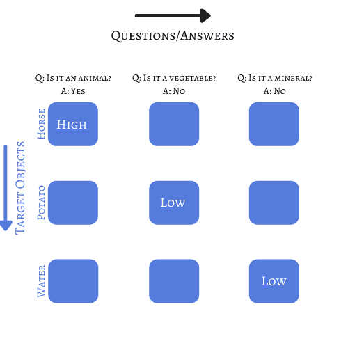
In further steps, the objects are ranked considering the given weight to each answer.
We might also have more options for answers such as “usually”, “sometimes”, “maybe”, and for each response, a respective weight can be assigned.
We can play its online version that can learn after each game is played, and, for this reason, it can guess correctly even after the player answered one question erroneously.
Before we dive into how the software can correctly guess the answer, we should understand the basics of one of the most used strategies to solve this problem and many others in Computer Science: Decision Trees.
Considering the used approach to learn parameters and achieve the desired goal, we can classify methods as parametric or nonparametric.
In parametric estimation, the parameters are learned considering the whole input space, and the model is built taking into account all the training data.
On the other hand, a nonparametric approach will divide the input space into smaller regions. Then, for each region, a local model will be computed using only the training data in that region.
A Decision Tree is a nonparametric hierarchical model that uses the divide-and-conquer strategy. It can be used for both regression and classification.
In supervised learning, we use decision trees to apply recursive splits in a region to break it into smaller regions. In this model, we have two types of elements, namely, decision nodes and terminal leaves.
Each decision done will contain a function  , and the output of this function will label the branches. So we should start at the root node and then iterate over the decision nodes, calculating
  to decide to each branch to go.
We do this recursively until we hit a leaf node. Once we reach a leaf node, the value written in that leaf is considered to be the output.
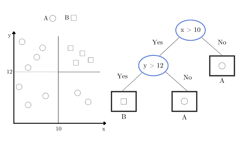
If we consider a hypothetical dataset with squares and circles, we’d have the corresponding decision tree, in which oval nodes are decision nodes, and rectangles are leaf nodes:
Another strong argument for us to consider the decision tree as a nonparametric model is the fact that we don’t presume the tree structure or the class densities, as they are defined over the learning phase and will depend on the complexity of the problem.
If our decision tree has multiple labels, we call it a classification tree. We can also calculate the impurity measure of our split, knowing that a split is considered pure if, for all branches, all elements belonging to a branch fit into the same class.
Considering that we have a node  , then
  will represent the number of elements reaching this node.
  is one element of that belongs to class
  . If we calculate the probability of the class at the node , we’d have:
(1) 
Considering that we’re at the node , if  is equal to 0 or 1 for all
  we consider this node to be pure. Consequently, either all elements belong to class or none of them belong.
For this reason, we should stop the splitting process since we reached a leaf. All elements with equals to  should receive the label .
But how can we classify the impurity if our node does not meet the requirements to be considered pure? First, we should understand the concept of entropy in information theory.
As Quinlan defined back in 1986, the entropy in information theory is the measurement of how many bits are required to encode the class code of an instance. Following the notation that we’re using since the beginning of this article, we can define an equation to calculate the entropy:
(2) 
In the next example, we’ll suppose that we have only 2 classes in our problem. In the first scenario we have  and
and  .
.
In this case, we have an entropy equal to 0 since all instances belong to  . We don’t need any bit since we won’t send anything.
But now let’s suppose we have  . In this scenario, we need 1 bit to identify which class is being used since they’re equally likely to occur.
We only evaluate the case with  classes equal to 2. Still, we can generalize for more complex applications, in the event of equal probabilities among the classes, that is
  :
:
(3) 
With this formula, we can define how many bits are necessary to encode all the classes in any problem.
Although the method mentioned previously can achieve high accuracy, different approaches can be used to solve the twenty questions challenge.
We can also combine different strategies to try to improve our model.
In our scenario, we have a classification tree since we’re trying to find the correct label among several options.
The leaves, in this case, will be the object or person that we’re trying to guess, and the branches will represent the features that led to one leaf, that is, the answers to the defined questions.
To understand the concept of Decision Tree, let’s consider a simpler version of the game, in which we only have four possible answers: dog, cat, carrot, and fork.
How many questions do we need to have in a game with 100% accuracy?
If we choose the questions carefully, with only two questions, we’ll be able to correctly guess the answer:
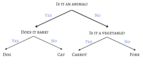
The previous example illustrates an optimal solution for a smaller version of the game in which we can find a word among four using only two questions.
Let’s mathematically define our problem considering what we discussed in section 3.3. If we have  possible choices of words, we can calculate the needed amount of questions
  :
:
(4) 
But if we know the number of questions, we can define how many different words we can correctly guess:
(5) 
So, for our 20 Questions Game, we have:
(6) 
With only 20 questions, we can identify more than one million different subjects, illustrating the effectiveness of using decision trees for this application.
We should highlight again that one of the most important aspects of this calculation is that we need to have an optimal set of questions capable of refining our answers, as illustrated in the example with four-word choices.
This optimal set of questions can be achieved by using some learning strategy. Ideally, each question would divide the possible answers in half, finding the main characteristics that separate the subjects.
Thus, our learning tree will work as a binary search, considering that the program recorded each played game and learned which questions provided the best results.
Together with the Decision Tree approach, we can add another strategy to our model. We can eliminate wrong answers by adopting the RANSAC strategy in which we randomly pick a subset of the 20 answered questions instead of all questions and verify which answer is given as output.
We do this several times with different subsets to check if the answer is the same in all of them.
This can help us prevent wrong answers given by the player from affecting the result since RANSAC is an outlier detection method, in which wrong answers will have their influence reduced in the final output.
In this article, we discussed how we could implement the 20 Questions Game using a nonparametric model called a decision tree.
With this structure, we’re able to solve many regression and classification problems. We also proved mathematically how we could predict the number of classes we can reach depending on the number of questions and how we can combine strategies to achieve higher accuracy.