What Is Cosine Similarity? | Baeldung on Computer Science

1. Overview

In this tutorial, we’ll talk about Cosine Similarity. First, we’ll define the term and discuss its geometric interpretation. Then, we’ll present some of its applications and an illustrative example.

2. Definition

Cosine similarity is employed as a measurement that quantifies the similarity between two or more non-zero vectors in a multi-dimensional space.

In this way, let’s suppose that we have two vectors $\mathbf{\vec{a} = (a_1, a_2, ..., a_n)}$ and $\mathbf{\vec{b} = (b_1, b_2, .., b_n)}$ in the n-dimensional space. To compute their cosine similarity, we compute the cosine of their angle $\mathbf{\theta}$ by calculating the dot product of the two vectors and dividing it by the product of their magnitudes. More formally, we have:

$\mathbf{sim (\vec{a}, \vec{b}) = cos (\theta) = \frac{\vec{a} \ \cdot \ \vec{b}}{||a|| \ \cdot \ ||b||}}$

Since the values of $cos (\theta)$ lies in the range $[-1, 1]$ , the similarity value has the following interpretations:

when $sim(\vec{a}, \vec{b}) = -1$ , we have strongly dissimilar vectors
when $sim(\vec{a}, \vec{b}) = 0$ , we have two orthogonal and independent vectors
when $sim(\vec{a}, \vec{b}) = 1$ , the vectors are strongly similar

All the intermediate values indicate the respective degree of similarity.

3. Geometric Interpretation

As we mentioned previously, the cosine similarity of two vectors comes from the cosine of the angle of the two vectors. Thus, now we will talk about the geometric interpretation of this similarity metric.

Let’s suppose that the angle between the two vectors is 90 degrees, meaning they have cosine similarity equal to 0. Geometrically, the vectors are perpendicular to each other, which indicates that these vectors do not have any relation.

As the angle of the vectors decreases from 90 to 0 degrees, the respective cosine similarity gets closer to 1, and the vectors become more and more similar. Next, we illustrate the geometric interpretation of cosine similarity using two examples.

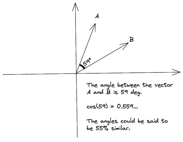
In the first diagram, the angle of our input vectors $\vec{A}$ and $\vec{B}$ is 59 degrees where $cos(59^{\circ}) = 0.559$ . So, the input vectors are 55% similar:

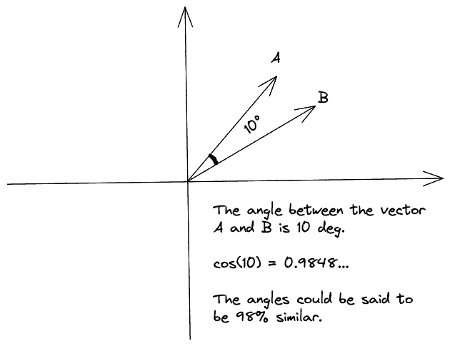
In the second diagram, we decrease the angle of the two vectors to 10 degrees. So, we have $cos(10^{\circ}) = 0.9848$ and the vectors are 98% similar:

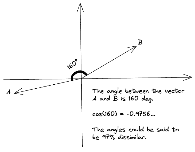
Finally, when the angle of the two vectors goes from 90 to 180 degrees, their cosine similarity decreases until it reaches the value of -1. In this scenario, the two vectors point in opposite directions, meaning they are strongly dissimilar. In the image below, we have $cos(160^{\circ}) = -0.9756$ and the vectors are 97% dissimilar:

4. Applications

The applications of cosine similarity are numerous. Let’s discuss the most important of them.

4.1. Information Retrieval

We often use cosine similarity in document retrieval systems where our goal is to find similar documents from a database. In this case, we have a query document represented by a semantic vector, and we compute its cosine similarity with a set of candidate documents. Also, we can group similar documents by clustering their vectors based on the similarity metric.

4.2. Natural Language Processing

Cosine similarity is very applicable in Natural Language Processing, where we often want to measure how semantically similar two words are. This information can be useful in tasks like sentiment analysis, text classification, and summarization.

4.3. Recommendation Systems

In recommendation systems, we often want to measure if two users prefer similar content. In this case, cosine similarity can be used to recommend similar items to these users.

4.4. Dimensionality Reduction

When working with high-dimensional data, it is very useful to plot some samples in 2 or 3 dimensions. So, dimensionality reduction methods are always explored to achieve a successful projection. In this context, cosine similarity can be used for preserving the similarity between the data points in the high and the low dimensional space.

5. Example

Finally, we’ll present an example of computing the cosine similarity between two vectors to illustrate the definition further.

Let’s suppose that we have two vectors $\vec{a} = (4, -3)$ and $\vec{b} = (-8, 6)$ . First, we compute their dot product as follows:

$\vec{a} \ \cdot \ \vec{b} = (4, -3) \cdot (8, 6) = 32 - 18= 14$

Then, we compute their similarity as follows:

$sim(\vec{a}, \vec{b}))= \frac{\vec{a} \ \cdot \ \vec{b}}{||a|| \ \cdot \ ||b||} = \frac{14}{5 \cdot 10} = \frac{14}{50} = 0.28$

So, the two vectors are 28% similar.

6. Conclusion

In this article, we talked about the cosine similarity metric. First, we presented the definition of the term and how we interpret it geometrically. Finally, we talked about some of its applications and discussed an illustrative example.

Full Archive

About Baeldung

Core Concepts

Operating Systems

Artificial Intelligence

Graph Theory

Latex