

Learn through the super-clean Baeldung Pro experience:
>> Membership and Baeldung Pro.
No ads, dark-mode and 6 months free of IntelliJ Idea Ultimate to start with.
Learn through the super-clean Baeldung Pro experience:
>> Membership and Baeldung Pro.
No ads, dark-mode and 6 months free of IntelliJ Idea Ultimate to start with.
In this tutorial, we’ll talk about computing the similarity between two colors. First, we’ll discuss the importance of having proper metrics for color similarity, and then we’ll present three methods for computing color similarity starting from the simplest to the most complex.
Nowadays, color modeling is an indispensable part of many applications, and colors are represented by a variety of color spaces like RGB, HSV, and HSL. The quantification of the similarity between colors is of great importance since it enables us to quantify a notion that was previously mostly described with adjectives.
As we’ll see below, computing color similarity is not a straightforward procedure since we cannot rely on classical proposed metrics to compare colors. Alternatively, we have to modify the equations of classical metrics in order to compute color similarity as perceived by humans.
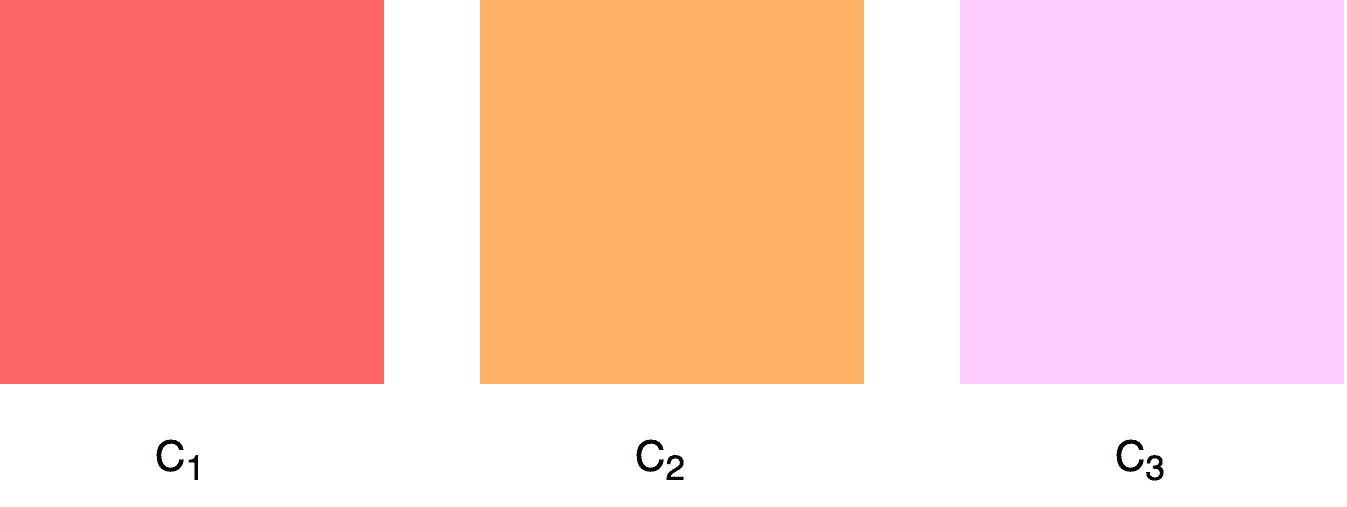
To better understand the below approaches, we’ll define three colors with RGB values  and
and  . Below, we can see the three colors:
The simplest approach is to apply a standard way of calculating distances in the RBG values of the color, like the Euclidean distance. For two given colors defined in RGB space as  and
and  , the euclidean distance is defined as:

In most cases, we can also avoid the square root and just compute the sum of differences between the RGB values.
If we apply the above equation in our previous colors we have:


That means that  is much closer to
  than
than  . However, this is not in accordance with our visual perception.
Despite its simplicity, this approach presents a serious flow since it does not account for the fact that humans perceive colors differently from the way colors are represented in the RGB color space. It is widely known that the human eye is more tolerant of some colors than others. So, visually similar colors may give us a greater RGB euclidean distance than colors that look much different to us.
An improvement to the above algorithm is to weigh RGB values to better fit human perception. The weights are computed experimentally, and the most common weights are 0.3 for Red, 0.59 for Green, and 0.11 for Blue.
So, the weighted euclidean distance distance between two colors defined in RGB space is defined as:

If we apply the above equation in our previous colors we have:


As before, is much closer to than but their difference is not so large.
Although weighted euclidean distance gives us a better estimate of color similarity, it is still not able to distinguish colors as humans do.
One of the best approaches to color similarity is to use the CIELAB color space that represents color using three values, namely:
 for perceptual lightness and
 and
and  for the four unique colors of human vision: red, green, blue, and yellow.
This model approximates very closely the way humans perceive colors where the component closely fits the human perception of lightness. So, the first step in computing color similarity is to convert the color from its original color space to CIELAB. This is usually very straightforward by applying some standard predefined equations. Then, we just compute the euclidean distance in the CIELAB space as follows:

where  and
and  are the values of the two colors in the CIELAB space.
This equation is a very good approximation of color similarity since colors are represented in the CIELAB color space that fits human perception.
Let’s apply this method to our example. First, we convert our three RGB colors to CIELAB as follows:


and then we compute their distances:


In this case, is closer to than since we took into account the way humans perceive colors.
In this article, we presented three methods for computing the similarity between colors. First, we discussed two simple approaches that are applied in the RGB color space.
Then, we talked about the best approach that computes the distance of colors in the CIELAB color space.