How to Calculate Receptive Field Size in CNN | Baeldung on Computer Science

1. Introduction

The receptive field of a convolutional neural network is an important concept that is very useful to have in mind when designing new models or even trying to understand already existing ones. Knowing about it allows us to further analyze the inner workings of the neural architecture we’re interested in and think about eventual improvements.

In this tutorial, we’re going to discuss what exactly a receptive field of a CNN is, why it is important and how can we calculate its size.

2. Definition

So what actually is the receptive field of a convolutional neural network? Formally, it is the region in the input space that a particular CNN’s feature is affected by. More informally, it is the part of a tensor that after convolution results in a feature. So basically, it gives us an idea of where we’re getting our results from as data flows through the layers of the network. To further illuminate the concept let’s have a look at this illustration:

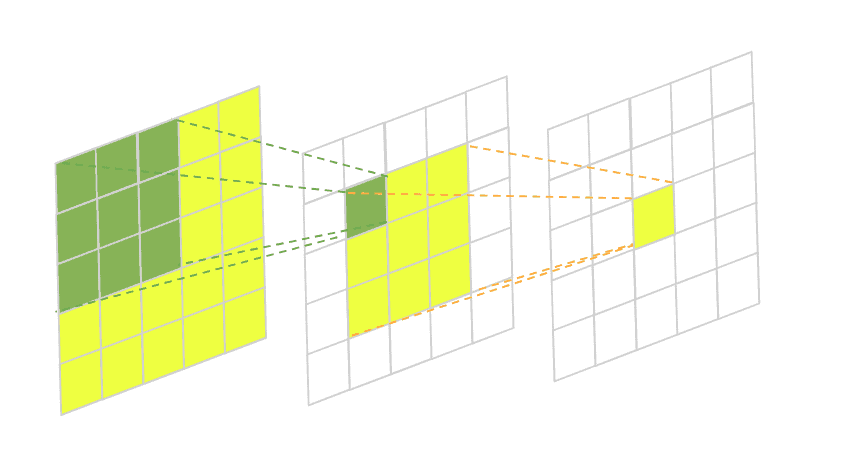
In this image, we have a two-layered fully-convolutional neural network with a 3×3 kernel in each layer. The green area marks the receptive field of one pixel in the second layer and the yellow area marks the receptive field of one pixel in the third final layer.

Usually, we’re mostly interested in the size of the receptive field in our initial input to understand how much area the CNN covers from it. This is essential in many computer vision tasks. Take, for example, image segmentation. The network takes an input image and predicts the class label of every pixel building a semantic label map in the process. If the network doesn’t have the capacity to take into account enough surrounding pixels when doing its predictions some larger objects might be left with incomplete boundaries.

The same thing applies to object detection. If the convolutional neural network doesn’t have a large enough receptive field some of the larger objects on the image might be left undetected.

3. Problem Explanation

3.1. Notation

We’ll consider fully-convolutional networks (FCN) with $L$ number of layers, $l=1,2,...,L$ . The output feature of the $l$ -th layer will be denoted as $f_l$ . Consequently, the input image will be denoted as $f_0$ and the final output feature map will correspond to $f_L$ . Each convolutional layer $l$ has its own configuration containing 3 parameters values – kernel size, stride, and padding. We’ll denote them as $k_l$ , $s_l$ and $p_l$ respectively.

Our goal is to calculate the size of the receptive field of our input layer $r_0$ . So how do we go about it? If we have a second look at the illustration above we might spot something like a pyramidal relationship between the size of the receptive field of the layers.

If we’re interested in the size of the base of the pyramid, we might describe it recursively using a top-to-bottom approach. What is more, we already know the size of the receptive field of the last layer – $r_L$ . It will always be equal to 1 since each feature in the last layer contributes only to itself. What is left is to find a general way to describe $r_{l-1}$ in terms of $r_l$ .

3.2. Simplified Example

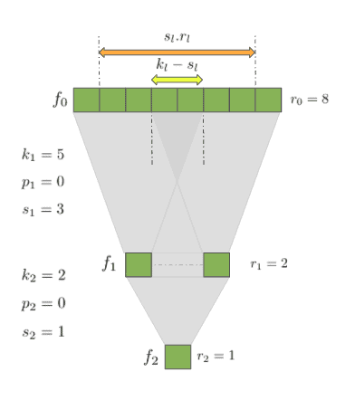
Let’s further simplify the problem and imagine our neural network as a stack of 1-dimensional convolutions. This doesn’t imply a loss of generality since most of the time the convolutional kernels are symmetric along their dimensions. And even if we work with asymmetric kernels we can apply the same solution along the dimensions separately. So here is our simple 1-d CNN:

If we look at the relationship between $f_2$ and $f_1$ it is pretty easy to see why the receptive field size is 2 – a kernel with size two is applied once. But when we go from $f_1$ to $f_0$ things start to get a bit more complicated.

3.3. Size Formula

We’d like to describe $r_{l-1}$ in terms of $r_l$ and come up with a general solution that works everywhere. As a start, let’s try and calculate $r_0$ in the above architecture. One good guess might be to scale $r_l$ by $s_l$ , denoted on the graph with the orange arrow. This gets us close, but not quite. We are not taking into account the fact that when the kernel size is different from the stride size we get a bit of a mismatch.

In our example $k_1=5$ and $s_1=3$ so there is a mismatch of $2$ denoted with the yellow arrow. This mismatch can generally be described as $k_l-s_l$ so that when $k_l >s_l$ we end up with an overlap like in the case of our $f_0$ . If it were the other way around and $k_l<s_l$ , there would have been a gap and $k_l-s_l$ will be negative. Either way, we would simply need to add this difference to the scaled receptive field of the current layer.

Doing so gives us the following formula:

$r_{l-1}=s_l.r_l+(k_l-s_l)$

We can apply the formula recursively through the network and get to $r_0$ . However, it turns out we can do better. There is another way to analytically solve the recursive equation for $r_0$ only in terms of $k_l$ ‘s and $s_l$ ‘s:

$r_{0}=\sum_{l=1}^{L}\left(\left(k_{l}-1\right) \prod_{i=1}^{l-1} s_{i}\right)+1$

The full derivation of this formula can be seen in the work of Araujo et. al.

3.4. Start and End Index Formula

Now that we can calculate the size of the region that affects the output feature map, we might also start thinking about which are the precise coordinates of that region. This might be useful when debugging a complex convolutional architecture, for example.

Let’s denote $u_l$ and $v_l$ the left-most and right-most coordinates of the region which are used to compute the feature in the last layer $f_L$ . We’ll also define the first feature index to be zero (not including the padding). Take for example this simple neural network, where $u_2 = v_2=0$ , $u_1=0$ , $v_1=1$ , and $u_o=-1$ , $v_o=4$ :

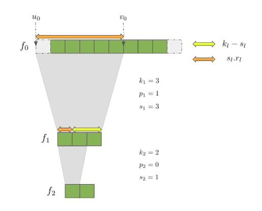To express the relationship between the start and end indices it might be again helpful to think recursively and come up with a formula that gives us $u_{l-1}$ , $v_{l-1}$ given $u_l$ , $v_l$ . Take for example the case when $u_l=0$ . Then $u_{l-1}$ will simply be the left-most index from the previous layer or $u_{l-1}=-p_l$ . But what happens when $u_l=1$ . Well, we’ll need to take the left-most index a stride away from $-p_l$ , meaning $u_{l-1}=-p_l + s_l$ . For $u_l=2$ the same calculation will be $u_{l-1}=-p_l + 2s_l$ and so on. This gives us the following formula:

$u_{l-1}=-p_{l}+u_{l} \cdot s_{l}$

To find the right-most index $v_{l-1}$ , we’ll just need to add $k_l-1$ :

$v_{l-1}=-p_{l}+v_{l} \cdot s_{l}+k_{l}-1$

4. Pseudocode

4.1. Finding the Receptive Field’s Size

It is pretty straightforward to use the analytical solution in order to calculate the receptive field of the input layer:

4.2. Finding the Receptive Field’s Start and End Indices

To find the start and end indices of a CNN’s receptive field in the input layer $u_0$ and $v_0$ we can simply use the above formulas and apply them:

5. Conclusion

In this article, we learned the receptive field of a convolutional neural network and why it is useful to know its size. We also took the time and followed through the derivations of a few very useful formulas for calculating both the receptive field size and location.

Full Archive

About Baeldung

Core Concepts

Operating Systems

Artificial Intelligence

Graph Theory

Latex