The Difference Between B-trees and B+trees | Baeldung on Computer Science

1. Introduction

In this tutorial, we’ll take a look at a type of data structure called a B-tree and a variation of it – B+tree. We’ll learn about their features, how they’re created, and how they’re used effectively in Database Management Systems for creating and managing indexes.

Finally, we’ll use the knowledge we’ve gained to compare B-trees and B+trees.

2. What Is a B-tree?

B-trees are a type of self-balancing tree structure designed for storing huge amounts of data for fast query and retrieval. They can be often confused with their close relation – the Binary Search Tree. Although they’re both a type of m-way search tree, the Binary Search Tree is considered to be a special type of B-tree.

B-trees can have multiple key/value pairs in a node, sorted ascendingly by key order. We call this key/value pair a payload. Occasionally we may hear the value part of the payload being referred to as “satellite data” or just “data”.

In the context of databases, a key may be the primary key or indexed column of a row, and the value could be the actual row record itself or a reference to it.

In addition to the payload, nodes also keep references to their children. Since each node typically takes up a disk page, these child references usually refer to the page ID in which the child node lives in secondary storage. As any search tree, B-trees are organized so that the keys of any sub-tree must be larger than the keys of the sub-tree to its left.

2.1. Properties of a B-tree

For a tree to be classified as a B-tree, it must fulfill the following conditions:

the nodes in a B-tree of order $m$ can have a maximum of $m$ children
each internal node (non-leaf and non-root) can have at least ( $m$ /2) children (rounded up)
the root should have at least two children – unless it’s a leaf
a non-leaf node with $k$ children should have $k-1$ keys
all leaves must appear on the same level

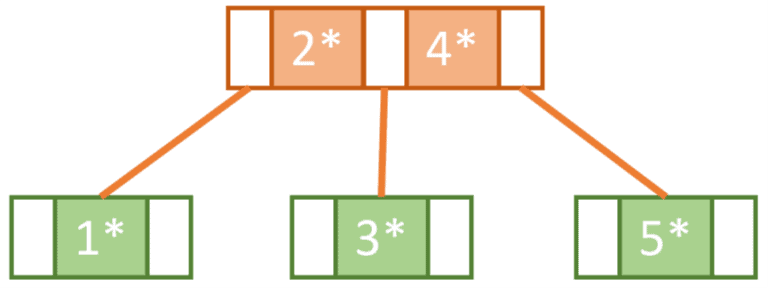
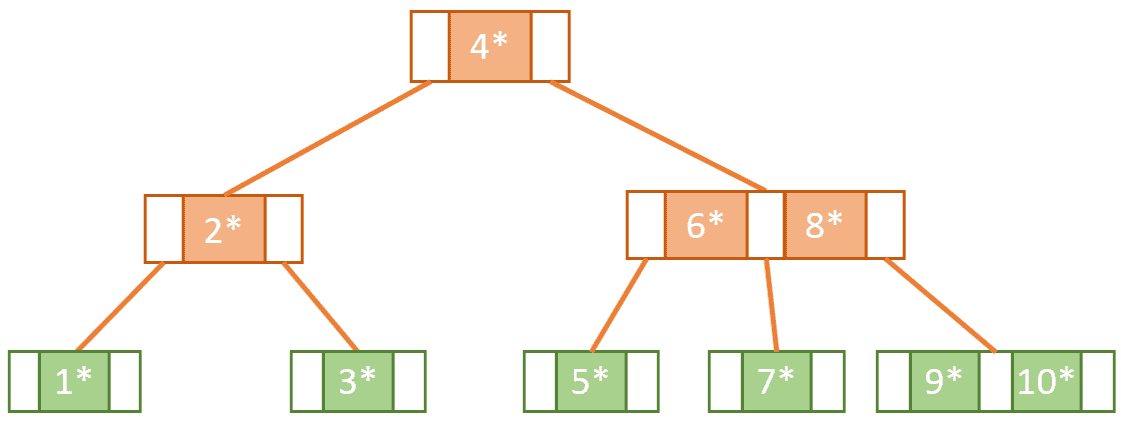
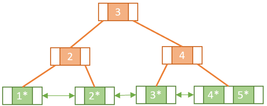
The image below shows us an example of a B-tree. The maximum number of children in this tree is 3, so we can conclude that this is a tree of order 3. All the leaves are on the same level, and the root and internal nodes have a minimum of two children fulfilling all the conditions of a B-tree:

2.2. Building a B-tree

Now, let’s build our tree from scratch. To do this, we’ll learn how to insert items into the tree while keeping it balanced.

Since we’re starting with an empty tree, the first item we insert will become the root node of our tree. At this point, the root node has the key/value pair. The key is 1, but the value is depicted as a star to make it easier to represent, and to indicate it is a reference to a record.

The root node also has pointers to its left and right children shown as small rectangles to the left and right of the key. Since the node has no children, those pointers will be empty for now:

We know that this tree has order of 3, so it can have only up to 2 keys in it. So we can add the payload with key 2 to the root node in ascending order:

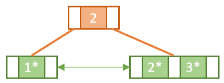
Next, if we wanted to insert 3, for us to keep the tree balanced and fulfilling the conditions of a B-tree we need to perform what is called a split operation.

We can determine how to split the node by picking the middle key. When we choose the middle key we need to consider the keys already present in the node and also the key which is to be inserted. In this case, 2 is the middle key used to split the node. This means the values to the left of 2 will go to a left sub-tree and the values to the right of 2 will go to a right sub-tree and 2 itself will get promoted as part of a new root node:

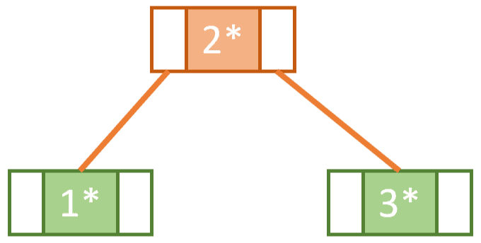
By performing this splitting operation each time we are about to exceed the maximum number of keys in a node, we keep the tree self-balancing.

Now, let’s insert 4. To determine where this needs to be placed we must remember that B-trees are organized such that sub-trees on the right have greater keys than sub-trees on the left. Consequently, Key 4 belongs in the right sub-tree. And since the right sub-tree still has the capacity, we can simply add 4 to it alongside 3 in ascending order:

Our right sub-tree is now at full capacity, so to insert 5 we need to use the same splitting logic explained above. We split the node into two so that Key 3 goes to a left sub-tree and 5 goes to a right sub-tree leaving 4 to be promoted to the root node alongside 2.

This rebalancing gives us space in the rightmost sub-tree to insert 6:

Next, we try to insert 7. However, since the rightmost tree is now at full capacity we know that we need to do another split operation and promote one of the keys.

But wait! The root node is also at full capacity, which means that it also needs to be split.

So, we end up doing this in two steps. First, we need to split the right nodes 5 and 6 so that 7 will be on the right, 5 will be on the left, and 6 will be promoted.

Then, to promote 6, we need to split the root node such that 4 will become a part of new root and 6 and 2 become the parents of the right and left subtrees:

Continuing in this way, we fill the tree by adding Keys 8,9 and 10 until we get the final tree:

2.3. Searching a B-tree

B-trees are considered to be so advantageous because they provide logarithmic $O(log(n))$ time complexity when it comes to insert, delete, and search operations.

Let’s take a look at how we would perform a search operation on our B-tree using the pseudocode below:

$\begin{minipage}{300} \begin{algorithm}[H] \SetAlgoLined \SetKwProg{FUNC}{Function}{:}{end} \FUNC{Search($node, searchKey$)} { i = 0\; \While{$i < node.Payloads.Count$ and $searchKey > node.Payloads[i].Key$}{ i++\; } \If{$searchKey = node.Payloads[i].Key$}{ \Return $node.Payloads[i].Value$\; } \If{$node.IsLeaf = true$}{ \Return null\; } \Return Search($node.Children[i]$, $searchKey$)\; } \caption{B-tree Search} \end{algorithm} \end{minipage}$

Our pseudocode assumes the following:

A node has an array of keys/value pairs node.Payloads and an array of references to its children nodes node.Children
The node object has a node.IsLeaf property which determines if its a leaf node or not
node.Payloads.Count refers to the number of payloads in a node

Let’s see how we can apply this pseudocode if we assume that the keys of our tree refer to IDs of a table, and we’d like to search for the record whose ID is 6. That means we’d be calling the Search method defined in the pseudocode with the parameters node = root node of the B-tree and searchKey = 6.

Using a while loop, we iterate through the root node keys increasing our counter value i until we find a key that is greater than or equal to 6 or until we have finished the keys of that node. The loop ends with i being at the value 1.

Now using i = 1 as an index, we select node.Children[1] (the child node at index 1). Iterating through its keys, we find node.Payload[0].Key to be an exact match to our searchKey. We end the search by returning node.Payload[0].Value, which is the satellite data associated with key 6.

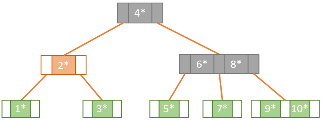
The image below shows our search path shaded in grey:

3. The B+tree

The most well-known version of the B-tree is the B+tree. What distinguishes the B+tree from the B-tree are two main aspects:

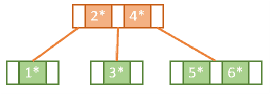
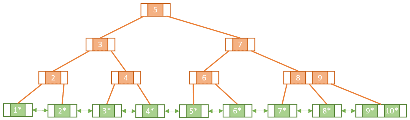
all leaf nodes are linked together in a doubly-linked list
satellite data is stored on the leaf nodes only. Internal nodes only hold keys and act as routers to the correct leaf node

Let’s see how our B-tree would look like if we were to represent its content as a B+tree:

Notice that some keys seem to be duplicated, like 2, 4, and 5. This is because, unlike leaf nodes, the internal nodes of a B+tree cannot hold satellite data and so we must make sure in some way that the leaf nodes include all the keys/value pairs.

Let’s build up our tree from scratch and see how this happens.

3.1. Building a B+tree

To start with, we’ll insert Keys 1 and 2 into the root node in ascending order:

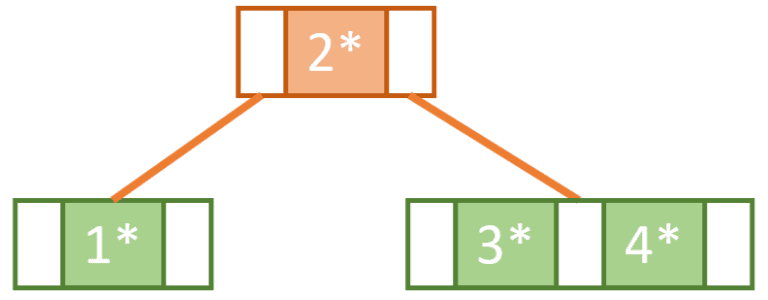
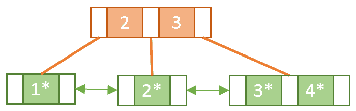
When we come to insert Key 3, we find that in doing so we will exceed the capacity of the root node.

Similar to a normal B-tree this means we need to perform a split operation. However, unlike with the B-tree, we must copy-up the first key in the new rightmost leaf node. As mentioned, this is so we can make sure we have a key/value pair for Key 2 in the leaf nodes:

Next, we add Key 4 to the rightmost leaf node. Since it’s full, we need to perform another a split operation and copy-up Key 3 to the root node:

Now, let’s add 5 to the rightmost leaf node. Once again to keep the order, we’ll split the leaf node and copy-up 4. Since that will overflow the root node, we’ll have to perform another split operation splitting the root node into two nodes and promoting 3 into a new root node:

Notice the difference between splitting a leaf node and splitting an internal node. When we split the internal node in the second split operation we didn’t copy-up Key 3.

In the same way, we keep adding the keys from 6 to 10, each time splitting and copying-up when necessary until we have reached our final tree:

3.2. Searching a B+tree

Searching for a specific key within a B+tree is very similar to searching for a key in a normal B-tree. Let’s see what it would be like to search for Key 6 again but on the B+tree:

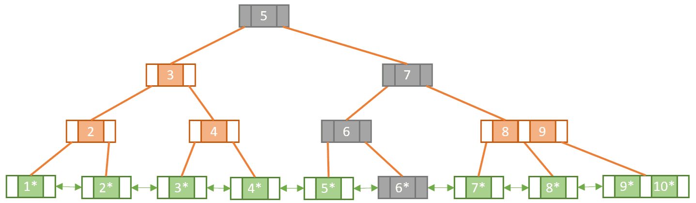
The shaded nodes show us the path we have taken in order to find our match. Deduction tells us that searching within a B+tree means that we must go all the way down to a leaf node to get the satellite data. As opposed to B-trees where we could find the data at any level.

In addition to exact key match queries, B+trees support range queries. This is enabled by the fact that the B+tree leaf nodes are all linked together. To perform a range query all we need to do is:

find an exact match search for the lowest key
and from there, follow the linked list until we reach the leaf node with the maximum key

4. B-trees in the Context of Databases

Storing and managing data is a fundamental part of computing. Main memory is considered to be a primary data storage, but we cannot store everything in it because it’s volatile and also expensive. That’s why we have secondary storage that’s less expensive and not volatile. Secondary storage is typically stored on magnetic disks in units called pages.

Transferring elements from disk to memory requires a read from the disk. A single disk read performs full-page access even if we are only trying to read one element from that page. Disk reads aren’t as fast as main memory reads since each time we do a read there it’s a seek and a rotational delay. The more disk accesses we need, the longer the search operation will take.

DBMSs leverage the logarithmic efficiency of B-tree indexing to reduce the number of reads required to find a particular record. B-trees are typically constructed so that each node takes up a single page in memory and they are designed to reduce the number of accesses by requiring that each node be at least half full.

5. Comparing Between B-trees and B+trees

Let’s cover the most obvious points of comparison between B-trees and B+trees:

In B+trees, search keys can be repeated but this is not the case for B-trees
B+trees allow satellite data to be stored in leaf nodes only, whereas B-trees store data in both leaf and internal nodes
In B+trees, data stored on the leaf node makes the search more efficient since we can store more keys in internal nodes – this means we need to access fewer nodes
Deleting data from a B+tree is easier and less time consuming because we only need to remove data from leaf nodes
Leaf nodes in a B+tree are linked together making range search operations efficient and quick

Finally, although B-trees are useful, B+trees are more popular. In fact, 99% of database management systems use B+trees for indexing.

This is because the B+tree holds no data in the internal nodes. This maximizes the number of keys stored in a node thereby minimizing the number of levels needed in a tree. Smaller tree depth invariably means faster search.

6. Conclusion

In this article, we took a close look at both B-trees and B+trees. We learned how they are built and how to search for a certain key.

Finally, with the information we learned, we were able to compare between the two in terms of structure, usage, and popularity.

Full Archive

About Baeldung

Core Concepts

Operating Systems

Artificial Intelligence

Graph Theory

Latex