

Learn through the super-clean Baeldung Pro experience:
>> Membership and Baeldung Pro.
No ads, dark-mode and 6 months free of IntelliJ Idea Ultimate to start with.
Learn through the super-clean Baeldung Pro experience:
>> Membership and Baeldung Pro.
No ads, dark-mode and 6 months free of IntelliJ Idea Ultimate to start with.
In this article, we’ll introduce amortized analysis as a technique for estimating run-time cost over a sequence of operations. We’ll step through two common approaches to evaluating amortized cost: the Aggregate Method and the Accounting Method.
Designing good algorithms often involves the use of data structures. When we use data structures, we typically execute operations in a sequence rather than individually.
If we want to analyze the complexity of a sequence like this, one simple approach might be to determine an upper bound on run-time for each individual operation in that sequence. Summing these values together, we can achieve an upper bound on the run-time of our entire sequence.
For some types of data structures, this approach may suffice. However, often the same operation will experience very different costs across a sequence. More specifically, sometimes an operation can only experience its worst-case cost on rare occasions.
In these cases, simply adding up the worst-case cost of individual operations may grossly over-estimate our actual runtime cost.
Amortization analysis attempts to solve this problem by averaging out the cost of more “expensive” operations across an entire sequence. More formally, amortized analysis finds the average cost of each operation in a sequence, when the sequence experiences its worst-case. This way, we can estimate a more precise bound for the worst-case cost of our sequence.
Let’s motivate this idea with an example – the dynamic array.
Consider an array A that starts off empty, with length N = 1 and number of elements n = 0. We can add an element to the end of the array, but whenever the array becomes full we need to automatically assign some more space.
So, after a couple of insertions, our array might look like this:
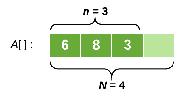
This type of data structure is called a dynamic array.
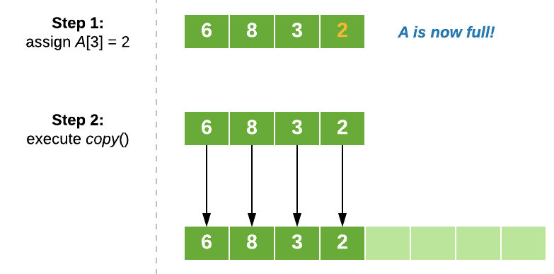
To add an element x to the end of our dynamic array, we call an operation called append(x).
append(x) has two steps:
copy() works by copying over each element from our previous array into a new array with twice the length.
Let’s visualize this operation with an example. Say we want to append the element “2” to our array A from above. Calling append(2) will trigger the following process:
If we want to analyze the worst-case cost of a series of append operations, we could simply sum up the individual worst-case cost of append,  , over the number of operations n. This will give us a bound of , which suggests that our performance will scale quite poorly.
However, this estimation is overly pessimistic.
Think about it this way, we’re assuming that every append operation in the sequence could call our copy function, which we know isn’t possible. append will only call copy when the array becomes full.
What we want to do instead, is determine the worst-case of our entire sequence and then find the average cost of each operation over this sequence.
This measure, called the amortized operation cost, will give us a much better indication of how well our append operation will actually perform.
As promised earlier, let’s take a look at two ways:
For this method, we apply a sum-and-divide approach, where we:
In other words:

Let’s apply this method to our dynamic array.
First, we need to determine the cost of each operation in the sequence. We’ll use Ci to denote the cost of the ith operation and assert that a simple assignment costs 1 unit of time.
We can start off by manually observing Ci for the beginning of our sequence:
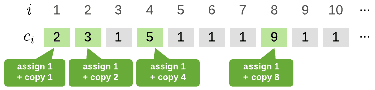
A pretty clear pattern is starting to emerge here. copy() is called whenever i is a factor of two, that is, when i = 1, 2, 4, 8, 16, … These operations will cost i units of time for copy, plus 1 unit of time for our simple assignment.
At every other position in the sequence, append will cost 1 unit of time.
Therefore, we can define Ci to be:
![\begin{align*} \[ C_i = \left\{\begin{array}{lr} i + 1, & \text{when } i \text{ is a power of 2}\\ 1, & \text{otherwise}\\ \end{array}\right. \] \end{align*}](/wp-content/ql-cache/quicklatex.com-2d7f5fc2e8764f6a89adaecf9e7128f8_l3.svg "Rendered by QuickLaTeX.com")
Now, to calculate T(n) we simply sum together each individual operation cost Ci in the sequence:

Now, we can simplify our last two summations to equal n, since together they they will occur exactly n times.

Finally, we can solve our first summation by recognizing that i can be a power of 2 at most log2n times in the sequence. So, we can transform this sum to have a new index j, which iterates over a range from 0 to log2n, and adds the value of 2j. If this step is a bit confusing, check out this page for a more detailed step through.

Finally, dividing by the number of operations n, we get:

As we can see, this method is very straight forward. However, it only works when we have a concrete definition of how much our sequence will cost.
Also, if our sequence contains multiple types of operations, then they will all be treated the same. We can’t obtain different amortized costs for different types of operations in the sequence. This might not be ideal!
Next, we’ll look at the Accounting Method, which can yield some more interesting results…
For this method, we think about amortized cost as being a “charge” that we assign to each operation.
Each time we encounter an operation, we try to pay for it using this “charge”.
If the operation actually costs less than our “charge”, we stash the change in a bank account. If the operation actually costs more than our “charge”, we can dip into our bank account to cover the cost.
The idea is that we want to save enough money during our “cheaper” operations to pay for any “expensive” operations we might encounter later on.
Let’s step through this method for our dynamic array.
For this analysis, we’ll use $1 to represent 1 unit of run-time. This means that our cheap append will cost $1 and our expensive append will cost $(i+1), where i is the position of this operation in the sequence.
So, how much should we charge each append operation?
This is the tricky part – we don’t want to charge too little or we’ll go broke trying to pay for our expensive operations. But we also don’t want to charge too much, as we’ll overestimate the cost needed to pay for our entire sequence.
This process requires a bit of abstract thought. While we’re becoming familiar with the process, one helpful approach is simple trial and error.
So, let’s start off by trying out a $1 charge. For this example, we’ll use B to denote our bank balance, and ΔB to denote the changes an operation makes to B:
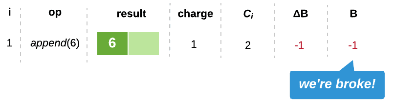
Clearly, this charge does not suffice. $1 will just cover the cost of a cheap append, with nothing saved to pay for our expensive operations.
How about charging $2?
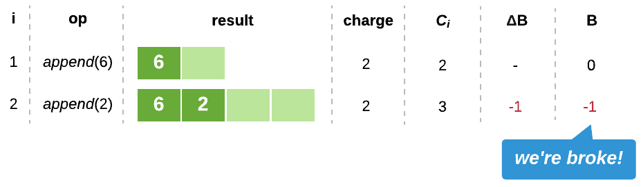
We can quickly see that charging $2 won’t suffice either.
What about $3?
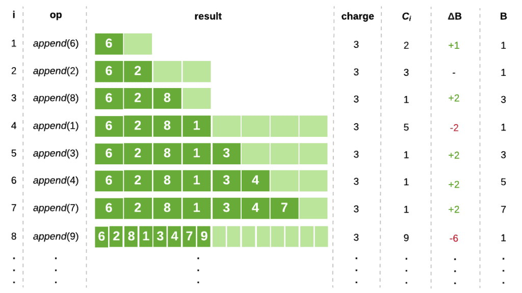
This looks promising! So far, our bank account hasn’t gone into deficit. And, as it turns out, charging $3 will guarantee the coverage of all future costs in our sequence.
We can prove this claim through simple induction.
First, we consider our initial copy, which occurs at position i = 0 and costs $2. Clearly, our charge will cover this cost.
Next, for our inductive case, we assume that our bank balance is >= 0 directly after an expensive append. Our array will now be half empty, which means that we must encounter N/2-1 cheap appends before another expensive append can occur.
If each of these operations saves $2 into the bank account, we will have at least $(N-2) saved. Along with our $3 charge, this will be sufficient to pay for our next expensive operation, which will cost $(N +1). Therefore, our bank account will not go into deficit.
Therefore, our $3 charge will cover all future costs in our sequence.
This means that our amortized operation cost has an upper bound of 3 =  .
.
Today, we focused our analysis on a sequence with just one type of operation. In this case, both the Aggregate and Accounting methods revealed the amortized cost for our append operation to be 3 = O(1).
However, if we instead analyzed a sequence with multiple types of operations, our results might not be so consistent.
The Aggregate Method will always treat every operation the same way, and cannot deduce different amortized costs for multiple types of operations in a sequence.
On the other hand, the Accounting Method can be easily applied to multiple operation types to deduce the amortized cost of each. To achieve this goal, we can simply assign a different charge to each operation type to reveal a unique amortized cost.
In this article, we introduced the concept of amortized cost analysis. We explored how amortized analysis can help us prove that a sequence of operations is actually quite efficient, even though its individual operations suffer an expensive worst-case cost.