

Learn through the super-clean Baeldung Pro experience:
>> Membership and Baeldung Pro.
No ads, dark-mode and 6 months free of IntelliJ Idea Ultimate to start with.
Last updated: March 18, 2024
Learn through the super-clean Baeldung Pro experience:
>> Membership and Baeldung Pro.
No ads, dark-mode and 6 months free of IntelliJ Idea Ultimate to start with.
In this tutorial, we’re going to investigate possible ways to solve a programming challenge. Given a series of towers of varying height, find the maximum amount of water that can be collected in the gaps between them.
Given a series of towers of varying height, water can collect between them up to the height of the tallest tower on either side. The question is to find this amount given an arbitrary set of towers to work with.
For example, given the following set of towers:
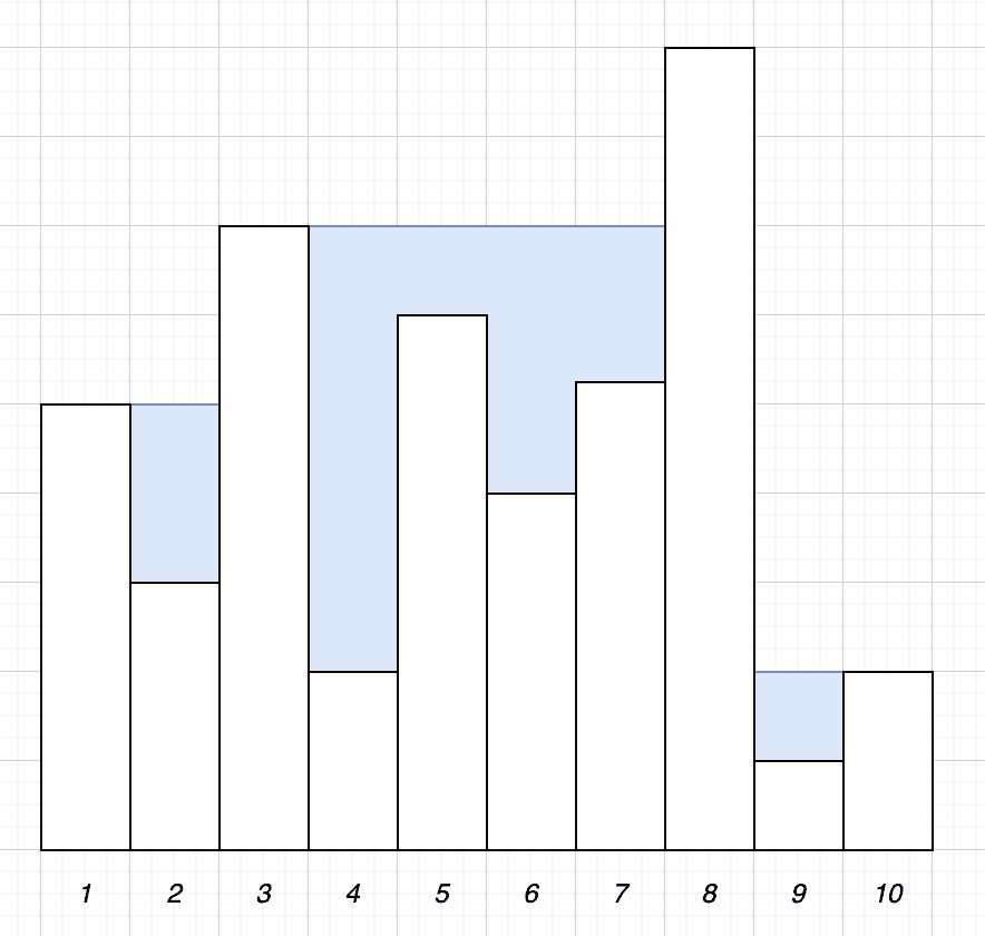
We have 14 units of water collected:
The naive solution is to simply count the amount of water that can be collected above each tower.
No water can be collected above the first and last tower. Any water that would be collected here will just drain off the outside of our towers. For all other towers, the amount of water is determined by whichever of the tallest towers to either side is shorter.
This sounds like a confusing concept, so we’ll understand what it means. In our above set of towers, let us take tower 2 as an example. Here we have a tower of height 3. To the left, we have a tower of height 5. No matter how tall the towers to the right are, water can never collect above level 5 because it will just drain off to the left.
Now that we understand this, our algorithm will be as follows:
algorithm NaiveAlgorithm(towers):
    // INPUT
    //    towers = an array representing the heights of the towers (0-based indexing)
    // OUTPUT
    //    water = the maximum amount of water that can be collected between the towers

    water <- 0

    for i <- 1 to len(towers) - 2:
        maxLeft <- 0
        maxRight <- 0

        for l <- 0 to i - 1:
            maxLeft <- max(maxLeft, towers[l])

        for r <- i + 1 to len(towers) - 1:
            maxRight <- max(maxRight, towers[r])

        minLeftRight <- min(maxLeft, maxRight)

        if minLeftRight > towers[i]:
            water <- water + (minLeftRight - towers[i])

    return water
Here we are iterating over every tower between the second and the second-to-last. For each of these, we’re then iterating over every tower to the left and then every tower to the right to find the tallest in each direction. We then take the shortest of these two sets. Once we have this, our amount of water is the difference between this tower and the one we are working with.
Once we’ve done this, we simply add these numbers up to get our total amount of water for this set of towers.
Now that we’ve seen the algorithm, let’s see how it works.
Starting with tower 2. First, we need to look at every tower to the left of it and determine which is the tallest – in this case, that’s tower 1, as it’s the only choice. Next, we need to look at every tower to the right and determine which of those are tallest – in this case, that’s tower 8:
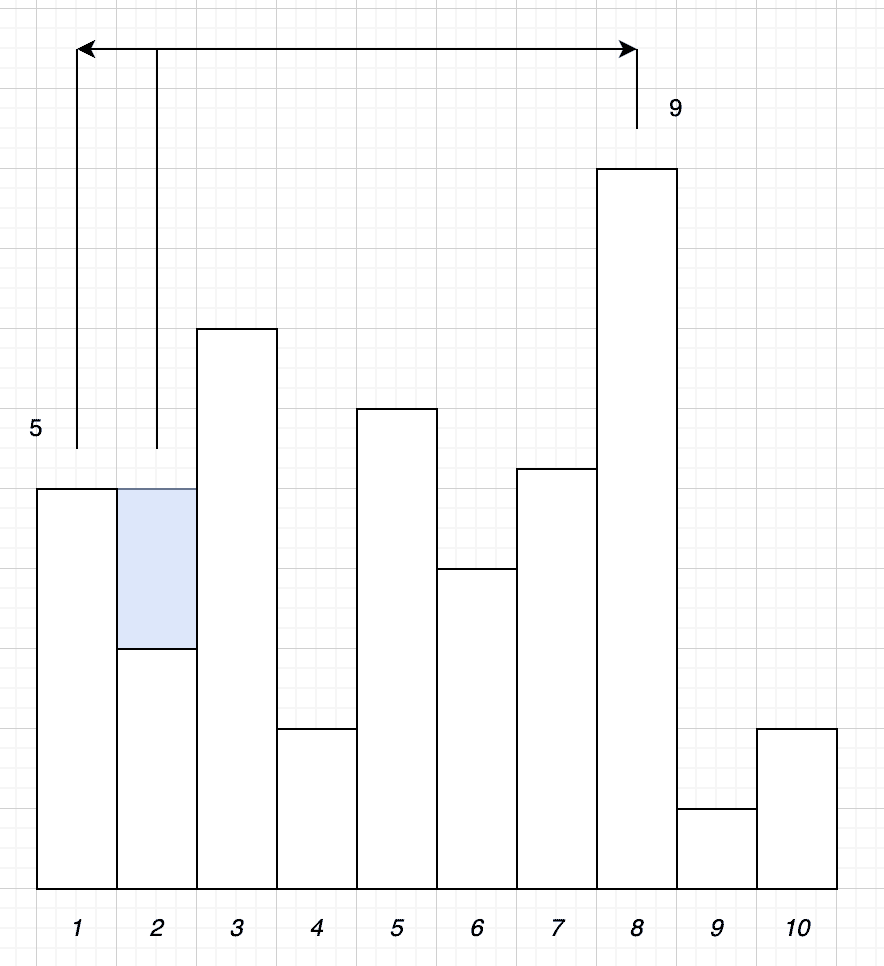
Out of these, tower 1 is shorter than tower 8. Finally, the difference in height between this and the tower that we are working with is 2 units – our tower is height 3, and tower 1 is height 5. This means that we can collect 2 units of water above this tower.
Next, we’ll look at tower 3. In this case, the tallest tower to the left is also tower 1, and the tallest tower to the right is also tower 8. However, in this case, tower 3 is taller than both of these, so there will be no water collected above it.
This algorithm is simple to understand but is very expensive. For our set of 10 towers, we are performing 17 loops and 88 comparisons.
In particular, we need to have 2(t – 2) + 1 loops. This is 1 overall loop, and then an additional 2 loops for every tower that we are looking at – which is each tower except for the first and last.
We then also need to have (t – 2)(t + 1) comparisons. Again, the (t – 2) portion is because we are examining every tower except the first and the last. The (t + 1) portion is actually made up of:
This gives us (t – 1 + 1 + 1) which is the same as (t + 1).
Our above solution works but is far from optimal. We can do better than this. By working out some details ahead of time, it’s possible to perform the exact same calculations with only two passes across the list of towers instead of needing 17.
Instead of calculating the local maximums every time we look at a new tower, we can instead calculate these and store the values. This is possible because the local maximum can never go down as we traverse the towers in the appropriate direction.
algorithm TwoPassAlgorithm(towers):
    // INPUT
    //    towers = a list representing the heights of the towers (0-based indexing)
    // OUTPUT
    //    water = the total amount of water that can be collected between the towers

    maxL <- an empty array
    currentMax <- 0

    for i <- 0 to len(towers) - 1:
        if towers[i] > currentMax:
            currentMax <- towers[i]
        maxL[i] <- currentMax

    water <- 0
    currentMax <- 0

    for i <- len(towers) - 1 to 0:
        if towers[i] > currentMax:
            currentMax <- towers[i]

        limit <- min(currentMax, maxL[i])

        if limit > towers[i]:
            water <- water + (limit - towers[i])

    return water
3.1. Algorithm in Action
As before, let’s look at this algorithm in action and see it working.
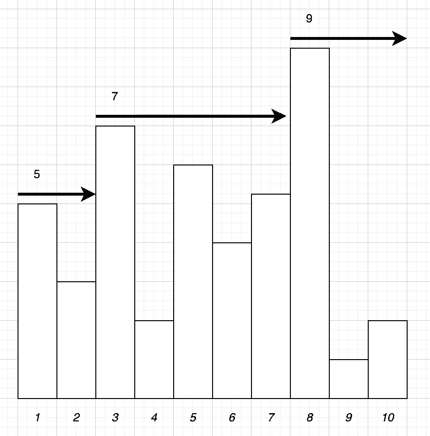
We work by making two passes across the list of towers. The first pass will build a list of numbers for each tower, recording the tallest tower to the left of this one. For example, towers 1 and 2 will record a value of 5, towers 3 to 7 will record a value of 7, and then towers 8 to 10 will record a value of 9:
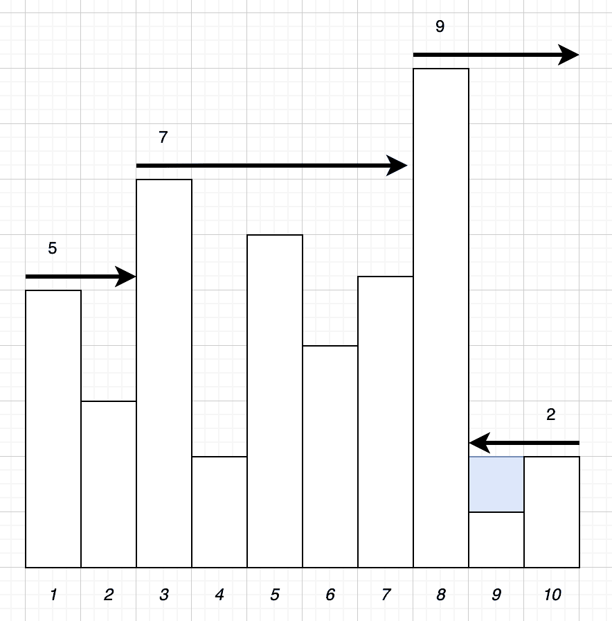
Next, we do the reverse, passing from right to left and recording the tallest tower so far. At each step, we can then use the previously recorded tallest tower to the left and the tallest tower we’ve seen on this pass from the right and calculate the amount of water above this specific tower.
If we look at tower 10, then our tallest to the left is height 9, and the tallest to the right is height 2. This means we compare this tower to height 2 and realize that there is no water collected above it.
Next, we look at tower 9. Our tallest tower to the left is still height 9, and the tallest to the right is still height 2. In this case, though, the current tower is height 1, so we are collecting 1 unit of water above it:
This time we will only ever need to have 2 iterations across the towers, no matter how many towers we have. However, this time we have 4t comparisons to make – 1 for each tower on our left pass, 1 for each tower on our right pass to track the current tallest, and an additional 2 for each tower on our right pass to calculate the amount of water above each one.
Comparing this to our first algorithm, we can see that this is cheaper as soon as we reach 6 towers on our list. This happens because the cost, in this case, is linear and not exponential.
However, it does come at another cost. In this case, we have to track additional data for each tower. We need a parallel array for tracking the tallest tower to the left of each one. So by significantly improving the time cost, we have instead had to pay for it with memory usage.
We also have a higher maintenance cost. This algorithm is more difficult to understand, and therefore will add an additional cost to future maintenance of our code.
Here we have looked at a specific problem – calculating the amount of water collected between towers. We’ve then looked at a couple of solutions to this, comparing them in terms of performance and maintenance complexity. Here we can see that there is always a trade-off between various things. We can make our algorithm perform better in some ways but always with a cost in other ways.
We should always strive to make our algorithms as good as possible, but we must consider everything when we do this. Sometimes we want to optimize for performance. Other times, we’re better off optimizing for maintenance instead. This choice will always depend on the exact circumstances of the project we are building.