Tabulation vs. Memoization | Baeldung on Computer Science

1. Introduction

In this tutorial, we’ll talk about tabulation and memoization as two techniques of dynamic programming.

2. Dynamic Programming

Dynamic Programming (DP) is an optimization paradigm that finds the optimal solution to the initial problem by solving its sub-problems and combining their solutions, usually in polynomial time. In doing so, DP makes use of Bellman’s Principle of Optimality, which we state as follows:

A sub-solution of the entire problem’s optimal solution is the optimal solution to the corresponding sub-problem.

So, DP first divides the problem so that the optimal solution of the whole problem is a combination of the optimal solutions to its sub-problems. But, the same applies to the sub-problems: their optimal solutions are also combinations of their sub-problems’ optimal solutions. This division continues until we reach base cases.

Therefore, each problem we solve using DP has a recursive structure that respects Bellman’s Principle. We can solve the problem by traversing the problem’s structure top-down or bottom-up.

3. Tabulation

Tabulation is a bottom-up method for solving DP problems. It starts from the base cases and finds the optimal solutions to the problems whose immediate sub-problems are the base cases. Then, it goes one level up and combines the solutions it previously obtained to construct the optimal solutions to more complex problems.

Eventually, tabulation combines the solutions of the original problem’s subproblems and finds its optimal solution.

3.1. Example

Let’s say that we have a $n\times n$ grid. The cell $(i,j)$ contains $c_{i,j}$ coins ( $i=1,2,\ldots, n; j=1,2,\ldots, n$ ). Our task is to find the maximal amount of coins we can collect by traversing a path from the cell $(1, 1)$ to the cell $(n, n)$ . In moving across the board, we can move from a cell to its right or bottom neighbor. We consider $c_{i,j}$ collected once we reach the cell $(i, j)$ .

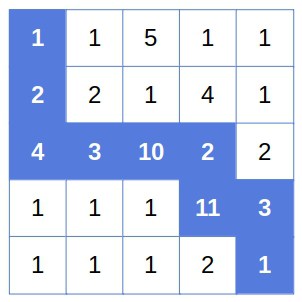
Here’s an example of a $5 \times 5$ grid, with the optimal path highlighted:

3.2. The Recursive Structure of the Problem

Let’s suppose that $P$ is the optimal path from $(1, 1)$ to $(n, n)$ and that it goes through cell $(i, j)$ . Then, the part of $P$ from $(1, 1)$ to $(i, j)$ , $P_{(1, 1) \rightarrow (i, j)}$ represents the optimal path between the two cells. If it wasn’t so, then there would be a better path $P'_{(1, 1) \rightarrow (i,j)}$ from $(1, 1)$ to $(i, j)$ . Consequently, $P$ wouldn’t be the optimal path to $(n, n)$ because the concatenation of $P'_{(1, 1) \rigtarrow (i, j)}$ and $P_{(i, j) \rightarrow (n, n)}$ would be better, and that would be a contradiction.

Now, let’s say that we’ve determined the optimal path $P$ to $(n, n)$ and its total yield $Y[t, n]$ . Based on the previous analysis and the problem definition, we conclude that $P$ must pass through $(n, n-1)$ or $(n-1, n)$ . So, the recursive definition of $Y[n, n]$ is:

$Y[n, n] = c_{n,n} + \max\{Y[n, n-1], Y[n-1, n] \}$

However, what holds for $Y[n, n]$ , also holds for any $Y[i, j]$ . When we account for the base cases, we get the recursive definition of $Y[i, j]$ :

(1) $\begin{equation*} Y[i, j] = \begin{cases} c_{1, 1}, & i=1 \text{ and } j=1\\ c_{1, j} + Y[1, j-1], & i=1 \text{ and } j > 1\\ c_{i,1} + Y[i-1, 1], & i>1 \text{ and } j=1\\ c_{i,j} + \max\{ Y[i-1, j], Y[i, j-1]\},& \text{otherwise} \\ \end{cases} \end{equation*}$

To reconstruct the path, we can use an auxiliary matrix $T$ where $T[i, j]=R$ if the optimal path reaches $(i, j)$ from the left (i.e., by moving one cell right from the predecessor cell), and $T[i,j] = D$ if it does so by moving one cell down. However, to keep things simple(r), we’ll omit path tracing and focus only on computing $Y$ .

3.3. The Tabulation Algorithm

Now, we reverse the direction of the recursion. We start from the base case $Y[1, 1]$ . From there, we find the yields of the paths to the cells in the $1$ st column and the first row. Then, we compute the values for the second column and row, and so on:

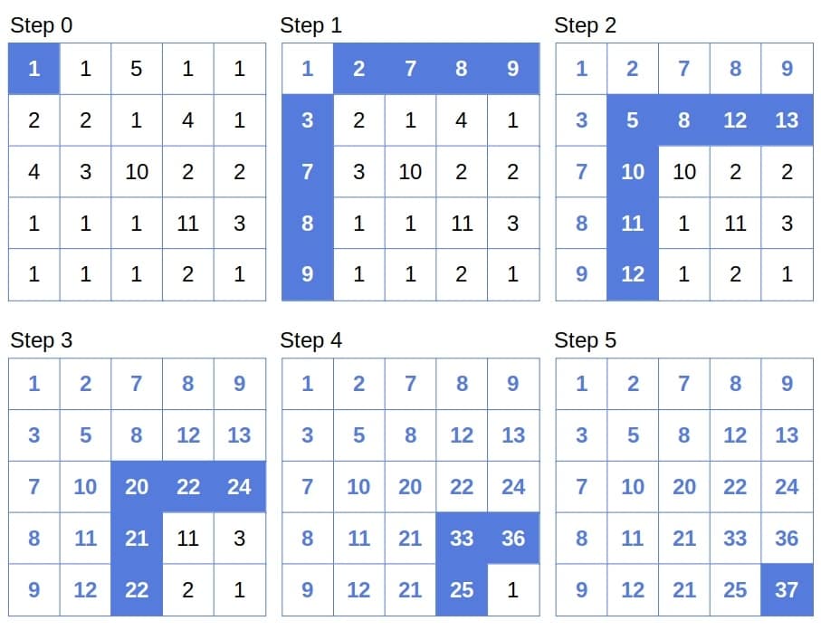
Processing the $\Gamma$ -shaped stripes one by one, we get our tabulation algorithm:

This algorithm’s time and space complexities are $O(n^2)$ .

3.4. The Anti-recursive Nature of Tabulation

Tabulation algorithms are usually very efficient. Most of the time, they’ll have polynomial complexity. And, since they’re iterative, they don’t risk throwing the stack overflow error. However, there are certain drawbacks.

First, we invest a lot of effort into identifying the problem’s recursive structure to get the recurrence right. However, the tabulation algorithms aren’t recursive. What’s more, they solve the problems in the reverse direction: from the base cases to the original problem. That’s the first drawback of tabulation. It may be hard to get the tabulation algorithm from a recursive formula.

Also, recursive relations such as (1) are natural descriptions of the problems to solve. So, they’re easier to understand than an iterative algorithm in which the recursive structure of the problem isn’t as apparent.

Finally, systematic in constructing more complex problems from the simpler ones, tabulation algorithms may compute the solutions to the sub-problems that aren’t necessary to solve the original problem.

4. Memoization

Is there a way to have the efficiency of tabulation and keep the elegance and understandability of recursion? Yes, there is, and it’s called memoization.

The idea behind it is as follows. First, we write the recursive algorithm as usual. Then, we enrich it with a memory structure where we store the solutions to the sub-problems we solve. If we reencounter the same sub-problem during the execution of the recursive algorithm, we don’t re-calculate its solution. Instead, we read it from memory.

This way, we avoid repeated computation and reduce the time complexity to the number of different sub-problems. We do so at the expense of the space complexity but don’t use more memory than the corresponding tabulation algorithm.

4.1. Example

Here’s the memoization algorithm for the grid problem:

This algorithm’s time and space complexities are $O(n^2)$ .

4.2. Memoization in Action

Let’s draw the first three levels of the memoization’s recursion tree:

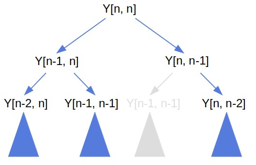
The algorithm calculates the value $Y[n-1, n-1]$ while computing $Y[n, n-1]$ in the root’s left sub-tree. Later, when it calculates $Y[n-1, n]$ in the right sub-tree, it doesn’t have to compute $Y[n-1, n-1]$ from scratch. Instead, it reuses the readily available value in the memory.

So, we see that memoization effectively prunes the execution tree.

4.3. Drawbacks of Memoization

Even though it’s intuitive and efficient, memoization sometimes isn’t an option. The problem is that it can cause the stack overflow error. That will be the case if the input size is too big. Iterative, the memoization algorithms don’t suffer from the same issue.

A more subtle but still relevant issue is related to the memory we use to store the results. For memoization to work, we need an $\boldsymbol{O(1)}$ -access memory structure. Hash maps, especially with double hashing, offer the constant worst-case access time. However, they require a hash function for the (sub-)problems. In the coin example, it’s easy to devise a quality hash. However, the problems may be complex, so a hash could be very hard to design.

Finally, some authors don’t consider memoization a DP tool, whereas others do. That isn’t a drawback by itself but is worth keeping in mind.

5. Conclusion

In this article, we talked about tabulation and memoization. Those are the bottom-up and top-down approaches of dynamic programming (DP). Although there’s no consensus about the latter being a DP technique, we can use both methods to obtain efficient algorithms.

While the memoization algorithms are easier to understand and implement, they can cause the stack overflow (SO) error. The tabulation algorithms are iterative, so they don’t throw the SO error but are generally harder to design.

Full Archive

About Baeldung

Core Concepts

Operating Systems

Artificial Intelligence

Graph Theory

Latex