

1. Introduction
When we process data, a common task is to be able to find the peak in an incoming signal.
For example, in a measured electrical signal, in seismic waves or wind speeds. We’re going to look into a few techniques to achieve this and why we’d want to use them.
2. Naive Processing
The simplest way to achieve this is to process our data and look for the highest spike. Often this is all that’s needed.
For example, given the stream of data:
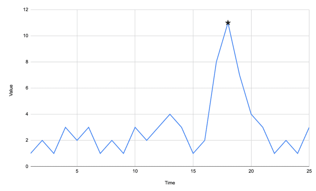
We can quickly process this data and find the peak at time 18.
This algorithm is a great fit where the peaks are significantly apparent in comparison to the background data. In our case above, the background data floats between 1 and 3, and our peak is at 11.
2.1. Algorithm
The algorithm is straightforward. We just look at each point in turn and record the highest one that we’ve seen so far.
When we reach the end of the data, the highest recorded value is then our peak:

3. Finding Multiple Peaks – Baseline
Our first algorithm works great if we’re looking for a single peak in relatively simple data. It doesn’t work at all if we’re looking for multiple peaks in the same signal, though – it will only be able to find the highest one.
For example, in the following signal:
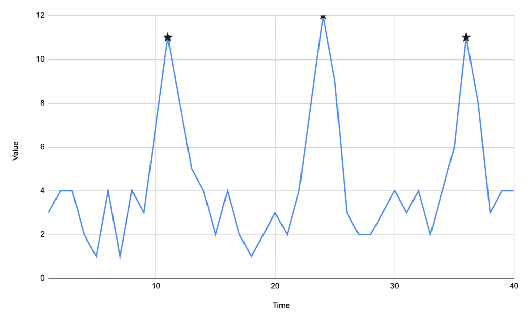
We can see that we have three prominent peaks, but our first algorithm will only find the one at time 24 – because it’s the one with the highest value.
One of the most straightforward options we have here is to generate a baseline. When we are processing our signal, if the current value ever drops below this baseline, then we can add our current peak to our outputs and then start again.
The easiest baseline to use is a simple mean of every value in our signal. In our above data, our mean is 4.325. Any time our signal drops below this value – which will happen at times 14, 26, and 38 – then we record our peak and start over.
3.1. Algorithm
The algorithm in this case is almost identical to the first one, only recording multiple peaks when needed:

4. Noisy Signals
Sometimes we have to process a signal where the noise level is significant compared to the signal itself. In these cases, the noise itself can give us many false positives and an incorrect result for finding peaks in the signal.
For example, the following signal is a sine wave only with added noise:
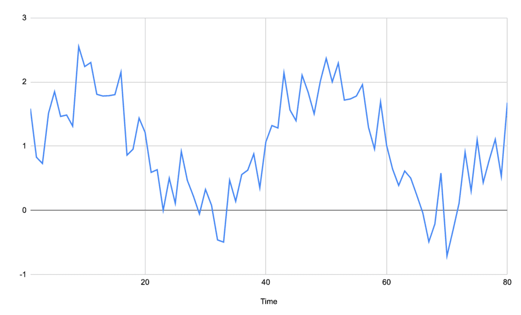
From this alone, it is challenging to see where the peaks would be. A baseline average like we saw before will not help because the noise is so great in comparison to the actual signal – in this case, there would be seven different peaks discovered in this signal when we expect only two.
Instead, we can calculate a moving average of the signal. Instead of a single value representing the entire data set, we can calculate an average for every single point that represents the surrounding points.
For example, if we were to take a moving average of two points either side, then the signal becomes:
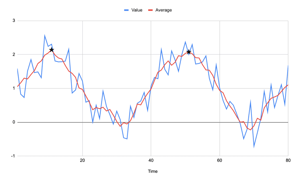
Immediately we can see much more clearly what the signal looks like and what the peak is.
Notably, the peaks on our new average signal don’t always correspond to peaks on the original signal, but they are always in the midst of the highest cluster of values.
4.1. Algorithm
The algorithm for this is very similar to before, but we now need to pre-process the signal before we find the peaks in it.

5. Detecting Wide Peaks
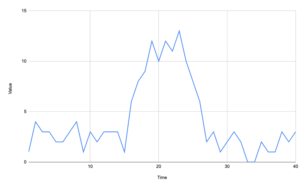
Everything we’ve looked at so far will detect a single high point in a signal. Sometimes this isn’t good enough, though. In some signals, we need to be able to detect a range of values that make up the entire peak. This is especially useful if we are looking for areas that the signal is considered “on”.
For example, in the following signal, there is a distinct area that is above the rest of the signal, and that entire range should be considered as the same peak:
This can be achieved by tracking every point above our baseline instead of just looking for the single highest one. We then need to adapt to handle the fact that a peak is a range of values now, not just a single one.
For example, if we track the peak of the above signal as being anything above the average of 4.2, then we get:
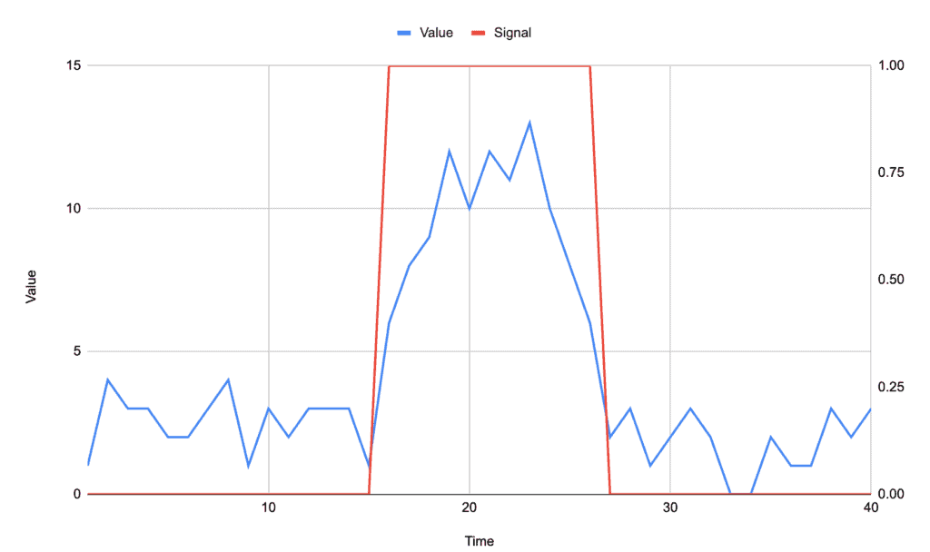
Depending on our exact needs, the actual desire might be to know the entire peak, or it might be to know the edges of the peak.
For example, if we are watching an electrical signal to detect a sensor being triggered, then we would want to know when a peak starts and ends, but may not care about the intervening period.
5.1. Algorithm
Many different algorithms can be adapted for this situation. In this case, let’s look at using an overall baseline to keep things simpler:

This simply returns every index that is above the baseline. It might be desired to return groups of indices that are above the baseline, where each group represents a single peak.
Alternatively, it might be that we want to convert the signal into a stream of high/low values instead of only pulling out the high values.
6. Dispersion by Standard Deviation
Dispersion is “the extent to which a distribution is stretched”. We can make use of this to detect when our signal is temporarily stretched more than usual. This can be done by tracking a moving average and looking for any points that are more than a certain number of standard deviations away from this.
The use of standard deviation here instead of just a straight baseline allows us to detect the difference between normal and abnormal peaks in the signal – where abnormal peaks are what we’re looking for.
For example, given the following signal:
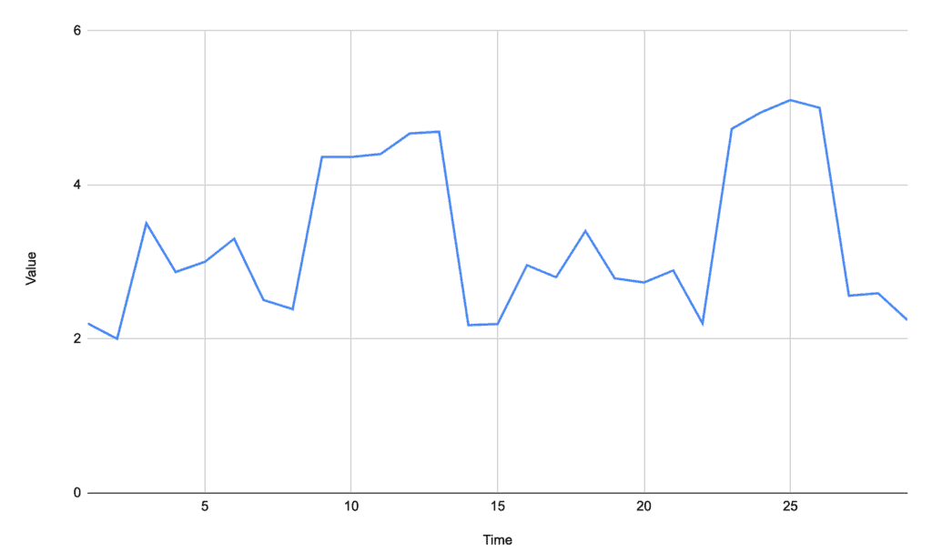
We have several small peaks above the baseline, but two very obvious ones that are what we’re looking to detect. A straight baseline would likely use the overall average of 3.29, which would also detect peaks at times of 3, 6, and 18.
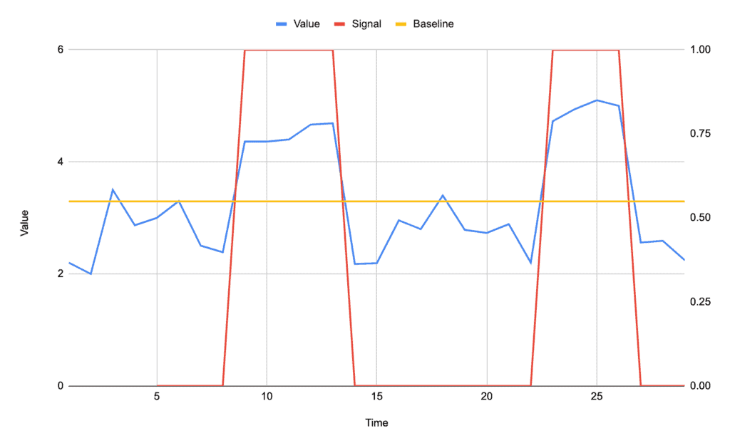
By using the dispersion algorithm, these are overlooked as not being significant, and instead, our two major peaks are the only ones detected:
6.1. Algorithm
This algorithm is more complicated than any of the earlier ones, but it has benefits for cases where it’s needed. We’re going to generate a moving baseline by calculating a new value for every point that is based off of a number of preceding points, and then we’re going to see how far the current point varies from this baseline:

This algorithm now has some other inputs, as well as the signal. We need to know:
- lag – the number of values before the current value that we want to use for computing the moving baseline.
- threshold – the number of standard deviations from the moving baseline that a peak needs to exceed to be counted.
- influence – the amount of influence that a peak has on the moving baseline. This must be between 0 and 1.
The algorithm compares each point to the average of the preceding lag points. However, when calculating this average, we adjust the values for any points that are considered to be a peak, because otherwise, they will distort what we want to see as the moving baseline.
The amount that we want to adjust these points by is called the influence and should be selected based on the expected size of our peaks compared to the base signal. The larger the peak, the less we want them to influence the moving baseline.
7. Summary
We’ve seen several different techniques here for detecting the peak in a signal, and there are many more that we haven’t looked at here as well.
The exact algorithm to use will depend on the signal that we are processing and what we need to get out of it.