Radix Sort | Baeldung on Computer Science

1. Introduction

In this tutorial, we’ll talk about Radix Sort, which is an $O(n)$ sorting algorithm.

2. Sorting in Linear Time

In a sorting problem, we have an array $a$ of $n$ objects and an ordering relation $\prec$ . Our goal is to sort $a$ so that each two consecutive elements $a[j]$ and $a[j+1]$ are in the correct order: $a[j] \prec a[j+1]$ .

When dealing with numbers, the relation $\prec$ is one of the $\{<, >, \leq, \geq\}$ . Here, we’ll assume the input array contains integers and should be sorted non-decreasingly, i.e., according to the relation $\leq$ . Also, we’ll use 1-based indexing.

Comparison sort algorithms sort the input by comparing their elements to decide their relative order. Such methods are, e.g., QuickSort and Merge Sort. The lower bound of the worst-case time complexity of all comparison sorts is $\Omega(n\log n)$ .

The Radix Sort algorithm, however, has linear time complexity.

3. Radix Sort

This algorithm sorts an array $\boldsymbol{a}$ of integers by sorting them on their digits from the least to the most significant one.

First, the algorithm sorts them by their least significant digits using Counting Sort. As a result, the numbers ending in 0 precede those ending in 1 and so on. Then, Radix Sort sorts the thus obtained array on the second-least significant digit, breaking ties by the order from the previous step. So, we must use a stable sort algorithm in each step.

The algorithm goes on like this until it sorts the numbers on the most significant digit. Once it does, the whole input array gets in the desired order.

3.1. Radix Sort in Action

Let’s take a look at an example:

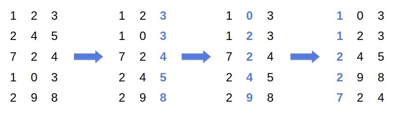
First, we sort the input on the least significant digit. Since $123$ is before $103$ in the original array, and the numbers end in the same digit, they remain in the same relative order after the first pass. Then, we sort the array on the middle digit, and finally, on the most significant one.

3.2. Complexity of Radix Sort

Assuming that the numbers have $d$ digits ( $0,1,\ldots, 9, A, B, C, \ldots$ ), Radix Sort loops $d$ times over $a$ . If the stable sorting algorithm it uses has the complexity $f(n)$ , then the time complexity of Radix Sort will be $O(df(n))$ .

In particular, Counting Sort is a linear-time non-comparison sorting algorithm. With it, Radix Sort’s complexity becomes $O(dn)$ , and if $d$ is a constant, the algorithm runs in $\boldsymbol{O(n)}$ time.

3.3. Pseudocode

Here’s the pseudocode of Radix Sort:

3.4. Proof

We can prove the correctness of Radix Sort by induction on $i$ . Our loop invariant is that the numbers we get by considering the $\boldsymbol{i}$ least significant digits are sorted for each $\boldsymbol{i}$ in the loop.

Since the invariant trivially holds before the loop, let’s show that if it’s true at the start of an iteration $i$ , it’s also true at its end. So, if each $a[j] = x_{d}^j x_{d-1}^j \ldots x_2^j x_1^j \equiv x_{d:1}^j$ , before the $i$ -th iteration starts, we have:

$x_{(i-1):1}^1 \leq x_{(i-1):1}^2 \leq \ldots \leq x_{(i-1):1}^n$

Now, we sort on the $i$ -th least significant digit. All the numbers whose digit in question is 0 are before the numbers that have one as their $i$ -th least significant digit, and so on. As a result, we conclude that if $\boldsymbol{x_i^{j_1} < x_i^{j_2}}$ , then $\boldsymbol{x_{i:1}^{j_1} < x_{i:1}^{j_2}}$ . So, to complete the proof, we need to show that the numbers with the same $\boldsymbol{i}$ -th least significant digit are in the non-decreasing order.

If $x_{i:1}^{j_1}$ and $x_{i:1}^{j_2}$ start with the same digit, and the former precedes the latter ( $j_1 < j_2$ ), then $x_{(i-1):1}^{j_1}$ preceded $x_{(i-1)}^{j_2}$ before the $i$ -th loop. That follows from the stability of Counting Sort. Since we assume the invariant held before the $i$ -th loop, we know that $x_{(i-1):1}^{j_1} \leq x_{(i-1):}^{j_2}$ . So, if $j_1 < j_2$ , then $x_{i:1}^{j_1} \leq x_{i:1}^{j_2}$ .

At the end of the loop, $i=d$ , so $a[j_1] \leq a[j_2]$ if $j_1 < j_2$ , which we wanted to prove.

4. Defining Digits in Radix Sort

We have some flexibility in defining the building blocks on which to sort. They don’t have to be digits. Instead, we can sort the numbers on groups made up from consecutive digits.

For example, we can break a $10$ -digit number into five words containing two digits each:

$x_9 x_8 \mid x_7 x_6 \mid x_5 x_4 \mid x_3 x_2 \mid x_1 x_0$

In general, if an integer has $b$ bits, we can write as a $\lfloor b/r \rfloor$ -digit word by grouping $r \leq b$ bits at a time. Then, the complexity of Counting Sort is $\Theta(n + 2^r)$ , and since we call it $d$ times, the complexity of Radix Sort is $\Theta \left(\frac{b}{r}(n+2^r) \right)$ . To get the best performance, we should set $r$ to the value that minimizes $\frac{b}{r}(n+2^r)$ .

If $b < \lfloor \log_2 n \rfloor$ , then $2^r \leq n$ since $r \leq b$ . So, in this case, setting $\boldsymbol{r=b}$ minimizes the expression.

Let’s suppose that $b \geq \lfloor log_2 n \rfloor$ . If we choose $r > \lfloor \log_2 n \rfloor$ , the $2^r$ term increases faster than $r$ , so the runtime is $\Omega \left( \frac{bn}{\log n}\right)$ . Setting $r$ to $\lfloor \log_2 n \rfloor$ makes the complexity $Theta \left( \frac{bn}{\log n} \right)$ . Using $r < \floor \log_2 n \rfloor$ increases the fraction $b/r$ while $n+2^r$ stays $\Theta(n)$ . So, $\boldsymbol{r=\lfloor \log_2 n \rfloor}$ is the optimal choice if $\boldsymbol{b \geq \lfloor log_2 n \rfloor}$ .

5. Radix Sort From the Most to the Least Significant Digit

We could sort the numbers on the digits from the most to the least significant one.

In the first pass, we sort $a$ on the most significant digit. Then, we recursively sort the sub-arrays containing the numbers starting with the same digit. In each call, we sort on the next less significant digit. When we sort on the last one, we stop.

Here’s the pseudocode:

However, the problem is that Counting Sort isn’t an in-place algorithm. Instead, it creates and returns a new array, that is, the input’s sorted permutation. So, recursive Radix Sort would reserve additional memory for $\boldsymbol{n}$ integers at each recursion level. Since the height of the recursive tree is $\boldsymbol{d}$ , this approach would take $\boldsymbol{\Theta(dn)}$ more memory than the first version of Radix Sort.

Even though that doesn’t change the algorithm’s space complexity if $d$ is a constant, it does affect memory consumption in practice. For that reason, recursive Radix Sort isn’t a good fit for applications with tight memory restrictions.

6. Sorting Non-integers

Can we apply this algorithm to non-integers? In general, the digits don’t have to be numerical. Any symbol (or a group thereof) can serve as a digit. However, we’d have to construct a mapping from actual to integer digits. The reason is that Counting Sort uses an integer array to count the elements.

Sometimes, Radix Sort isn’t applicable even if we design an integer mapping. For example, let input objects have $10$ fields, each with millions of possible values ( $k$ ). Although $d=10$ , there are too many digits. Consequently, Counting Sort will perform poorly, taking way more memory than needed.

We could use a hash map to reduce memory consumption, but we’d need to design a quality hash function. But, since hashed values would change over time, the worst-case complexity of hash lookup would be $O(k)$ . So, the approach would still be inefficient in practice.

7. Conclusion

In this article, we presented Radix Sort. It’s a stable linear-time sorting algorithm. Although Radix Sort has a linear time complexity, the multiplicative coefficient hiding under $\Theta(n)$ makes it less efficient than asymptotically worse comparison sorts in practice. Also, since Counting Sort isn’t an in-place algorithm, Radix Sort may take more memory than an $\boldsymbol{O(n\log n)}$ algorithm such as Quick Sort.

Full Archive

About Baeldung

Core Concepts

Operating Systems

Artificial Intelligence

Graph Theory

Latex