Linearly Separable Data in Neural Networks | Baeldung on Computer Science

1. Introduction

In this tutorial, we’ll explain linearly separable data. We’ll also talk about the kernel trick we use to deal with the data sets that don’t exhibit linear separability.

2. Linearly Separable Classes

The concept of separability applies to binary classification problems. In them, we have two classes: one positive and the other negative. We say they’re separable if there’s a classifier whose decision boundary separates the positive objects from the negative ones.

If such a decision boundary is a linear function of the features, we say that the classes are linearly separable.

Since we deal with labeled data, the objects in a dataset will be linearly separable if the classes in the feature space are too.

2.1. Linearly Separable 2D Data

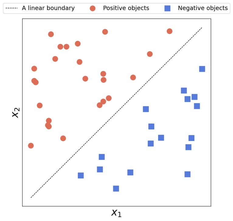
We say a two-dimensional dataset is linearly separable if we can separate the positive from the negative objects with a straight line.

It doesn’t matter if more than one such line exists. For linear separability, it’s sufficient to find only one:

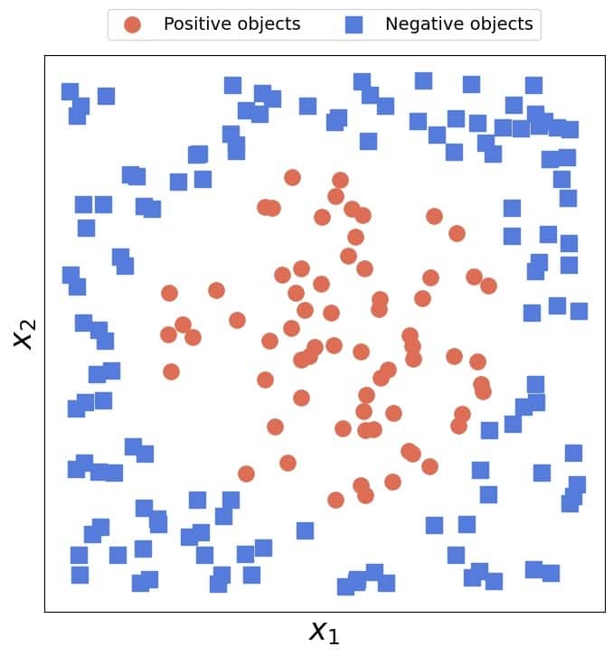
Conversely, no line can separate linearly inseparable 2D data:

2.2. Linearly Separable $n$ -Dimensional Data

The equivalent of a 2D line is a hyperplane in $n$ -dimensional spaces. Assuming that the features are real, the equation of a hyperplane is:

(1) $\begin{equation*} \sum_{i=1}^{n} w_i x_i + b = \langle \mathbf{w}, \mathbf{x}\rangle + b = 0 \quad \mathbf{w}=[w_1,w_2,\ldots w_n], \mathbf{x}=[x_1, x_2, \ldots, x_n], b \in R \end{equation*}$

where $\langle \cdot, \cdot \rangle$ is the dot product (that also goes by the name of inner product) and $\mathbf{w}$ is the vector orthogonal to the hyperplane. $\mathbf{x}$ stands for an object from the feature space.

2.3. Linear Models

If the data are linearly separable, we can find the decision boundary’s equation by fitting a linear model to the data. For example, a linear Support Vector Machine classifier finds the hyperplane with the widest margins.

Linear models come with three advantages. First, they’re simple and operate with original features. So, it’s easier to interpret them than the more complex non-linear models. Second, we can derive analytical solutions to the optimization problems that arise while fitting the models. In contrast, we can rely only on numerical methods to train a general non-linear model. And finally, it’s easier to apply numerical methods to linear optimization problems than non-linear ones.

However, if the data aren’t linearly separable, we can’t enjoy the advantages of linear models.

3. Mapping To Linearly Separable Spaces

In such cases, there’s a way to make data linearly separable. The idea is to map the objects from the original feature space in which the classes aren’t linearly separable to a new one in which they are.

3.1. Example

Let’s consider as an example the 2D circular data from above. No straight line can separate the two classes faultlessly. However, while that’s true in the original 2D space with features $x_1$ and $x_2$ , mapping to another could make the objects separable. Let’s see if that’s true for the mapping:

$\begin{bmatrix} x_1 \\ x_2 \end{bmatrix} \mapsto \begin{bmatrix} x_1 \\ x_2 \\ x_1^2 + x_2^2 \end{bmatrix}$

Since all the data points with $x_3 = x_1^2 + x_2^2 \leq b$ are positive for $b$ equal to the positive circle radius while the rest are negative, the transformed data will be linearly separable. So, we can fit a linear SVM to the transformed set and obtain a linear model of $x_1$ , $x_2$ , and $x_3$ conforming to Equation (1).

3.2. Issues

This approach has several issues. First, we have to design the mapping manually. Sometimes, the correct transformation isn’t straightforward to come by. That’s usually the case when we deal with complex data. Additionally, there may be multiple ways to make the data linearly separable, and it’s not always clear which one is the most natural, the most interpretable, or the most efficient choice. For instance, all these mappings make the circular data from above linearly separable:

$\begin{bmatrix} x_1 \\ x_2 \end{bmatrix} \mapsto \begin{bmatrix} x_1 \\ x_2 \\ \sqrt{x_1^2 + x_2^2} \end{bmatrix} \qquad \begin{bmatrix} x_1 \\ x_2 \end{bmatrix} \mapsto \begin{bmatrix} \sqrt{x_1^2 + x_2^2} \end{bmatrix} \qquad \begin{bmatrix} x_1 \\ x_2 \end{bmatrix} \mapsto \begin{bmatrix} x_1^2 + x_2^2 \end{bmatrix} \qquad \begin{bmatrix} x_1 \\ x_2 \end{bmatrix} \mapsto \begin{bmatrix} (x_1^2 + x_2)^{\frac{1}{100}} \end{bmatrix}$

Another problem is that transforming the data before fitting the model can be overly inefficient. If the dataset is large and the transformation is complex, mapping the whole set to the new feature space could take more time and memory than we can afford.

Finally, if the data become linearly separable only in an infinite-dimensional space, we can’t transform the data as the corresponding mapping would never complete.

To solve these issues, we apply the kernel trick.

4. Kernels

Let’s go back to Equation (1) for a moment. Its key ingredient is the inner-product term $\langle \mathbf{w}, \mathbf{x} \rangle$ . It turns out that the analytical solutions to fitting linear models include the inner products $\langle \mathbf{x}, \mathbf{z} \rangle$ of the instances in the dataset.

When we apply a transformation mapping $\Phi$ , we change the inner-product terms in the original space to the inner products in another one: $\langle \Phi( \mathbf{x} ), \Phi( \mathbf{z} ) \rangle$ . But, we can evaluate them even without transforming the data. To do so, we use kernels.

A kernel $k$ is a function that maps a pair of original objects $\mathbf{x}$ and $\mathbf{z}$ into the inner product of their images $\Phi( \mathbf{x} )$ and $\Phi( \mathbf{z} )$ without actually calculating $\Phi( \mathbf{x} )$ and $\Phi( \mathbf{z} )$ . So, kernels allow us to skip the transformation step and find a linear decision boundary in another space by operating on the original features.

For example, $k \left( [x_1, x_2], [z_1, z_2] \right) = x_1^2 z_1^2 + 2 x_1 z_1 x_2 z_2 + x_2^2 z_2^2$ is the inner product of $[x_1^2, \sqrt{2 x_1 x_2}, x_2^2]$ and $[z_1^2, \sqrt{2 z_1 z_2 }, z_2^2]$ . So, if the separating decision boundary in the original space is a curve involving the terms $x_1^2$ , $x_2^2$ , or $\sqrt{x_1 x_2}$ , it will be a plane in the transformed space. Therefore, training a linear model kernelized with $k$ will find it.

5. Conclusion

In this article, we talked about linear separability. We also showed how to make the data linearly separable by mapping to another feature space. Finally, we introduced kernels, which allow us to fit linear models to non-linear data without transforming the data, opening a possibility to map to even infinite-dimensional spaces.

Full Archive

About Baeldung

Core Concepts

Operating Systems

Artificial Intelligence

Graph Theory

Latex