

1. Introduction
In this tutorial, we’ll examine the class of metaheuristic algorithms inspired by various natural elements. This will require us to understand what metaheuristics are and why we need them for solving optimization problems. This will help us to explore the inspirations coming from nature. We’ll go through the details of some of the popular nature-inspired algorithms and their applications.
2. Optimization Problems and Metaheuristics
In mathematics and engineering, an optimization problem is a problem of finding the best solution from all feasible solutions. We usually define such a problem as an objective function of one or more variables with a set of constraints. These problems can be discrete or continuous, depending upon whether the variables involved are discrete or continuous.
The complexity of an optimization problem directly relates to the objective function and the number of variables it considers. Interestingly, many real-world optimization problems fall into a category known as NP (Non-deterministic Polynomial-time). It means that we can solve them in polynomial time with a non-deterministic algorithm:
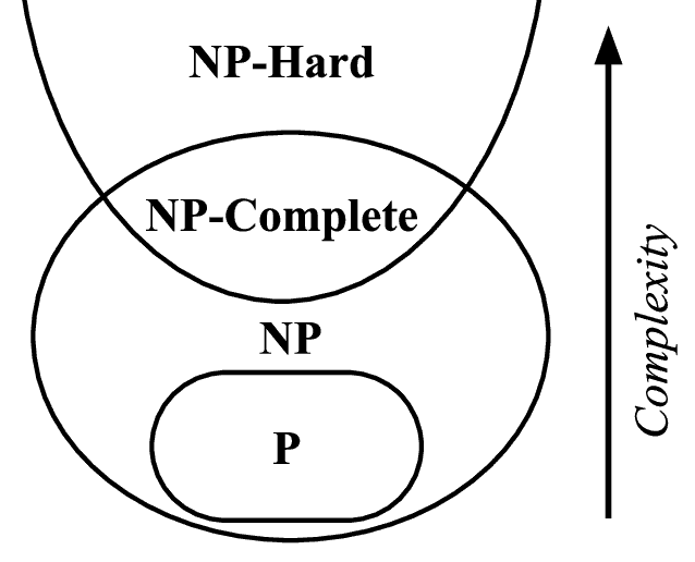
A detailed analysis of NP or NP-hard problems is beyond the scope of this tutorial. However, it’s sufficient to understand that finding the globally optimal solution for such problems would require many resources. Hence, it becomes practically infeasible or at least inefficient. Many common problems like traveling salesman and graph coloring fall into this category.
This is where a metaheuristic can help us. A metaheuristic is a higher-level procedure or heuristic that can provide a sufficiently good solution to an optimization problem. Typically they operate by sampling a subset of solutions that are too large to be completely enumerated. Most importantly, they can also work with incomplete or imperfect information.
Unlike numerical optimization algorithms, a metaheuristic can not guarantee that it will find the globally optimal solution. However, it can achieve reasonable solutions quicker with far less computational effort. Many metaheuristics also employ stochastic optimization, where the solutions they find depend upon random variables.
3. Formulating the Metaheuristic
The goal of a metaheuristic is to explore the search space to find the near-optimal solutions efficiently. They are based on a strategy to drive the search process. The strategy can take inspiration from any natural or artificial system under observation. This can come from as diverse sources as the metallurgical process of annealing to the foraging behavior of ants.
Defining a metaheuristic around a search strategy requires us to pursue scientific and engineering goals. The scientific goal is to model the mechanism behind an inspiration like a swarm of ants. The engineering goal is to design systems that can solve practical problems. While it’s impractical to define a generic framework, we can discuss some defining characteristics.
One of the key aspects of any metaheuristic approach is to strike the right balance between exploration and exploitation. The objective of exploration is to explore as much of the feasible region as possible to evade sub-optimal solutions. The objective of exploitation is to explore the neighborhood of a promising region to find the optimal solution.
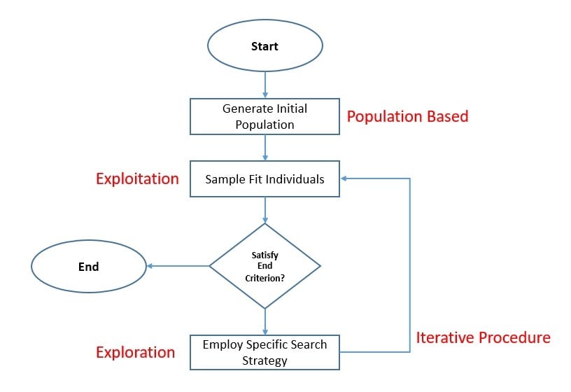
Almost in all such metaheuristics, we tend to employ a fitness function to evaluate the candidate solutions. This is to sample the best solutions so far to focus on exploitation. Further, we use certain aspects of the search strategy to bring randomness and emphasize exploration. This is unique to every search strategy and hence quite difficult to represent using a general formulation.
We can use these metaheuristics to solve multi-dimensional real-values functions without relying on their gradient. This is an important point as it implies that we can use these algorithms for solving optimization problems that are non-continuous, are noise, and change over time. This is contrary to several algorithms that use gradient descent, like linear regression.
4. Types of Nature-inspired Metaheuristics
Over the years, a lot of research has gone into developing novel metaheuristic techniques. We have seen that strategies that drive the search process can be quite diverse, resulting in a broad spectrum of metaheuristic algorithms. Hence, it’s difficult to classify them meaningfully. One such attempt to classify metaheuristics is documented here:
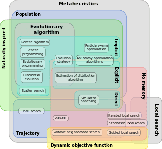
The focus of this tutorial is nature-inspired metaheuristics. These are metaheuristics whose search strategy is inspired by natural systems. Above is an Euler diagram to classify different metaheuristics based on local vs. global search and single vs. population-based search properties.
Evolutionary computation forms a subfield of artificial intelligence with a family of global optimization algorithms inspired by biological evolution. We can classify nature-inspired metaheuristics using their inherent properties in multiple ways. Although, we’ll particularly focus on a class of nature-inspired metaheuristics known as Evolutionary Computation (EC).
There is a complex classification of algorithms within Evolutionary Computation. However, we’ll focus on a board classification of Evolutionary Computing into Evolutionary Algorithms (EA) and Swarm Algorithms (SA). They both use the population-based presentation of the candidate solutions and an iterative procedure with stochastic exploration.
4.1. Evolutionary Algorithms
Evolutionary Algorithms (EA) is a class of algorithms inspired by Darwin’s evolutionary theory. Darwin’s evolutionary theory postulates that the variation occurs randomly among members of a species. It also suggests that its progeny could inherit an individual’s traits, and the struggle for existence would allow only those with favorable traits to survive.
Evolutionary algorithms take inspiration from this theory to identify near-optimal solutions in the search space. Each iteration in such an algorithm is known as a generation and is composed of parent selection, recombination (crossover), mutation, and survivor selection. While crossover and mutation are responsible for the exploration, parent and survivor selection brings out the exploitation.
4.2. Swarm Algorithms
Swarm Algorithms (SA) are inspired by the collective behavior of social animals and insects. A swarm consists of multiple agents, like bees. The behavior of a single agent is extremely simple, local, and stochastic. Even without a centralized structure to control the agent behavior, interactions between agents produce global intelligent behavior, called Swarm Intelligence (SI).
These algorithms take inspiration from the collective behavior of natural agents like ants or bees. The key point in such algorithms is the information shared within the swarm, which can directly influence the movement of each agent. By controlling the information sharing between agents in a swarm, we can achieve the balance between exploration and exploitation of the search space.
5. Popular Evolutionary Algorithms
Since the beginning of Evolutionary Computing (EC) several decades earlier, a lot of focus has been on evolutionary algorithms. Intensive research into this area resulted in mature algorithms like Genetic Algorithm (GA), Genetic Programming (GP), Evolutionary Programming (EP), and Differential Evolution(DE). In this section, we’ll discuss the details of a few popular Evolutionary Algorithms (EA).
5.1. Genetic Algorithm
The genetic algorithm is perhaps one of the oldest and the most popular nature-inspired metaheuristic we know today. It was introduced back in 1975 by John Holland as a search optimization algorithm based on the mechanics of the natural selection process. At the core, it tries to mimic the concept of “the survival of the fittest”, where the strong tend to adapt and survive while the weak tend to perish.
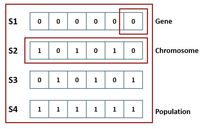
An individual solution in the problem domain is genetically represented as a chromosome. We characterize a solution by a set of parameters called genes. Then, we join all the genes into a string to form a chromosome:
We start by selecting an initial population either randomly or using some heuristic. Then we use a fitness function to evaluate the population members and rank them on their performance. This leads to the elimination of lower rank chromosomes. The remaining population goes on to participate in the process of reproduction:
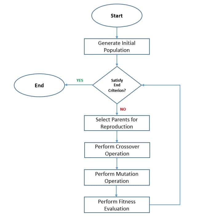
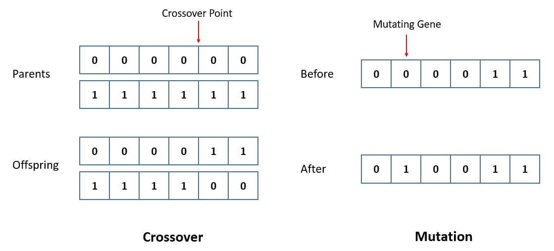
The following two operators, crossover and mutation, are crucial for the genetic algorithm. The crossover randomly selects two chromosomes from the population and mates them by exchanging their genes. The mutation consists of taking a chromosome and randomly mutating its gene. These operators allow the algorithm to emphasize exploration of the search space:
The cycle repeats, and the generation of a new population continues until the end criterion is met. This is either by reaching the maximum number of generations or finding the optimal solution. We can also use other strategies to allow lower-rank chromosomes to participate in reproduction. Further, we can employ elitism to prevent the best solution from being destroyed during crossover and mutation.
5.2. Differential Evolution
The differential evolution is another very popular algorithm in evolutionary algorithms. It’s quite similar in technique to the genetic algorithm and was introduced way back in 1997 by Rainer Storn and Kenneth Price. The key difference lies in how differential evolution uses mutation as the primary operator in searching for better solutions.
As with the genetic algorithm, we begin by selecting an initial population and then evaluating individual solutions’ fitness. The algorithm utilizes mutation operation as the search mechanism and selection operation to direct the search toward the potential regions:
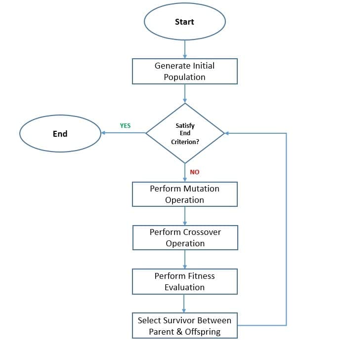
There are three parameter vectors to generate the new population in each iteration. We select these parameter vectors randomly from the current population. During the mutation step, we generate a mutant or donor vector by utilizing the first parameter vector called the base vector and a difference vector created from the other parameter vectors:
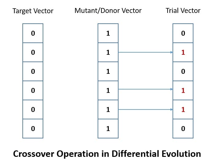
Then we perform a crossover between the target vector and the mutant vector to produce the trial vector. Here, the target vector contains a solution in the search space. Finally, we select by picking between the target vector (parent) and the trial vector (offspring) based on the fitness function of the problem domain.
Unlike the genetic algorithm, all solutions in the population have the same probability of being selected as the parent. The offspring is only evaluated after the mutation and crossover operations. Moreover, the offspring in differential evolution is discarded immediately if it does not perform better than the parent. It results in preserving the best-so-far solution individually.
6. Popular Swarm Algorithms
Swarm Algorithms (SA) are relatively new in Evolutionary Computing (EC) and are a very active area of research. We can read about new metaheuristics in the literature inspired by the collective behavior of new agents like Salp Swarm and Grey Wolf. However, we’ll restrict ourselves to a few popular algorithms in this area, like Ant Colony Optimization (ACO) and Particle Swarm Optimization (PSO).
6.1. Ant Colony Optimization
Ant Colony Optimization is one of the earliest and most widely studied and adopted metaheuristics in the swarm intelligence category. Marco Dorigo proposed it in his doctoral thesis way back in 1992. The foraging behavior of ants inspires it. More specifically, it tries to mimic the way ants can find the shorter paths between their colony and food sources using pheromone.
An ant drops a chemical called pheromone over the path it travels. When other ants find a pheromone trail, they tend to follow it. However, over time pheromone evaporates and reduces in intensity. Now, a short path than a longer path gets traveled more frequently. Thus, the pheromone intensity on shorter paths becomes higher than on the longer ones:
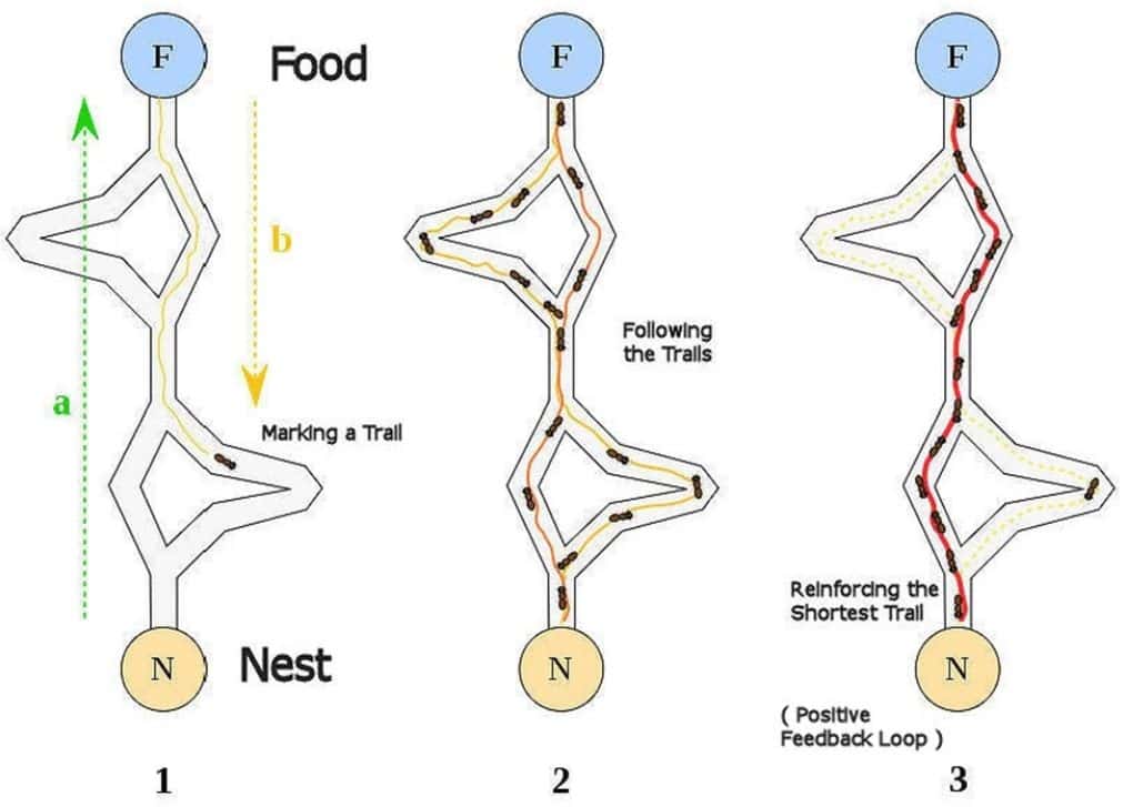
We need to transform the optimization problem into the problem of finding the shortest path on a weighted graph. We use ants as imaginary agents in the ant colony algorithm to explore and exploit the search space. In an iteration of the algorithm, each artificial ant tries to stochastically construct a solution by finding the order in which to traverse the edges of the graph:
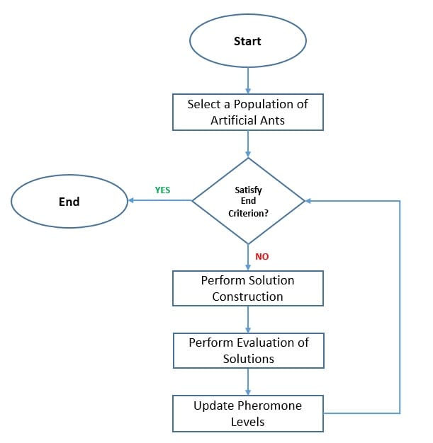
Then, we compare the path constructed by the different ants and update the pheromone levels on each edge accordingly. This plays an important role in the way ants select an edge in their solution. They consider the length of each edge from their current position and their corresponding pheromone level to arrive at a decision.
The pheromone updates happen through deposit and evaporation. According to the evaluation value, the artificial ants increase the pheromone on their trail, and the pheromone decreases over time. The difference between deposit and evaporation keeps a balance between exploration of the search space by artificial ants and the exploitation of optimal solutions.
6.2. Particle Swarm Optimization
Another very popular metaheuristic in the category of swarm intelligence algorithms is Particle Swarm Optimization. It was introduced by J. Kennedy and R. Eberhart in 1995, almost after the introduction of Ant Colony Optimization. It takes inspiration from the simple swarming behavior of natural agents, like the flocking of birds and the schooling of fish.
The algorithm begins by selecting a population of candidate solutions known as particles. Then it involves moving these particles around in the search space according to simple rules based on the particle’s position and velocity. The movement of particles is influenced by parameters like their own best-known position (pbest) and the entire swarm’s best-known position (gbest):
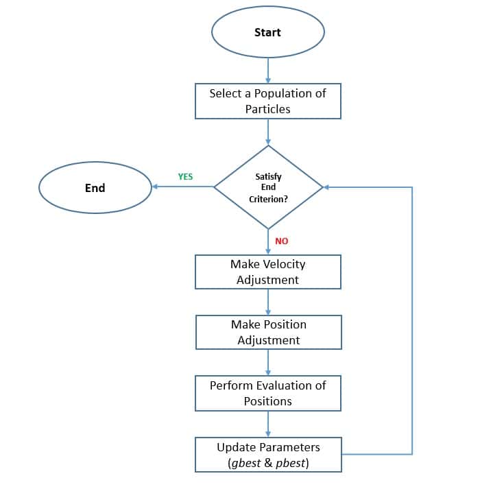
Here, the global best solution is an element that promotes the convergence of the swarm to the optimal locations. At the same time, the personal best solution of each particle contributes to the maintenance of swarm diversity by generating unique behavior for each particle. These parameters are also important in updating the velocity of each particle, considering their inertia.
A useful intuition behind how particle swarm optimization works is to understand in terms of a few simple behaviors. For instance, we can describe this with behaviors like separation, alignment, and cohesion:
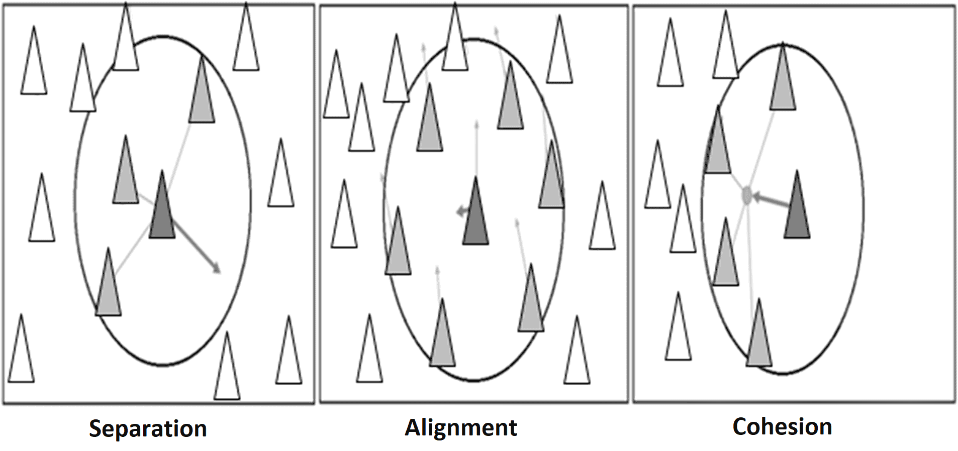
Here, separation is the behavior of avoiding crowded local flockmates. Alignment is the behavior of moving towards the average direction of the local flockmates. Finally, cohesion is the behavior of moving towards the average position of the local flockmates. With this, the algorithm can maintain a balance between exploration of the search space and exploitation of the optimal solutions.
7. Other Interesting Algorithms
As we’ve seen earlier, the field of metaheuristics is at least five decades old, but it remains an active area of research. This is primarily because no metaheuristic can claim to solve all the optimization problems. As we encounter more interesting real-world optimization problems, our quest for a better metaheuristic propels the research in this field.
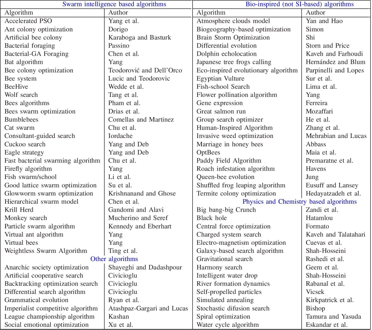
So far, we’ve focussed on the metaheuristics inspired by the biological agents of nature. But, the field of nature-inspired metaheuristics is much wider than that. This can include natural agents from other areas of study, like chemistry, and physics. For instance, gravity, river formation, electromagnetism, and the black hole, to name a few from one of the literature reviews:
While much high-quality research has been done in this area, most literature remains largely experimental. While the literature claims novelty and practical efficacy, they may not prove to be practical for real-world engineering problems. It’s for us to do a rigorous exercise to understand their value. Nevertheless, we should continue to invest and improve in metaheuristics.
There have been several attempts to classify metaheuristics in the past, including the one presented in this tutorial. However, it’s essential to understand that they are valuable only to a certain extent, and we should not get hung up on them. There is a lot of cross-over between the areas of study that inspires a metaheuristic and hence it’s bound to be quite complex.
8. Practical Applications
As we’ve seen earlier, the reason behind a surge of interest in metaheuristics is to solve real-world optimization problems that are otherwise difficult to solve. We often come across optimization problems in engineering and other domains that present a vast and difficult search space. To find a helpful solution in such cases, using traditional approaches prove to be inefficient.
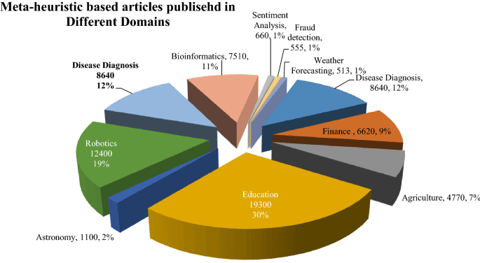
Since the early days, metaheuristics have been successfully applied to solve some well-known combinatorial problems, like the traveling salesman problem. We have also seen applications of these algorithms in a wide range of domains, like education, robotics, medical diagnosis, sentiment analysis, finance, fraud detection to name a few:
It’s important to note that a metaheuristic takes very few assumptions about the optimization problems. Hence, they apply to a vast variety of problems. But, at the same time, it does not guarantee the same level of performance for all these problems. Hence, we must make specific alterations in the algorithm to make it more suitable for particular problems.
This has resulted in numerous variations of the common nature-inspired metaheuristics that we’ve seen in this tutorial. It’s much beyond the scope of this tutorial to even name all of them! Further, a lot of research goes into fine-tuning the parameters of each of these algorithms that can make them suitable for a specific problem domain.
Finally, it’s important to note that while we’ve developed a lot of intuition behind these algorithms, they largely work like black boxes. So, it’s challenging to predict which algorithms in some specific form can work better for an optimization problem. As we keep discovering new problems and demand better performance for existing ones, we’ve to keep investing in research!
9. Conclusion
To sum up, in this tutorial, we went through the basics of nature-inspired metaheuristics and why we even need them. Although the spectrum of these algorithms is quite wide, we focussed on some of the well-known algorithms in the category of evolutionary algorithms and swarm algorithms. Finally, we discussed some of the practical applications of these metaheuristic algorithms.