Jump Search Algorithm | Baeldung on Computer Science

1. Introduction

In this tutorial, we’ll present the Jump Search algorithm.

2. Search Problems

In a classical search problem, we have a value $z$ and a sorted array $x$ with $n$ elements. Our task is to find the index $i$ of $z$ in $x$ .

If $x$ is a linked list, it doesn’t have indices. Instead, each element is a $(key, item)$ pair, so we’re looking for the item whose key is $z$ . We’ll denote the $i$ th element of the list $x$ as $x[i]$ just as we do with arrays.

However, if $x$ is an array, we can access any element in an $O(1)$ time (assuming that $x$ fits into the main memory). In contrast, if $\boldsymbol{x}$ is a list, we need to follow $\boldsymbol{i-1}$ pointers to reach $\boldsymbol{x[i]}$ , so the complexity of access is $O(i)$ . In the worst case, we want to reach the end of the list, so we traverse all the $n$ elements to get to it, which takes $O(n)$ time.

That’s why an array search algorithm such as Binary Search isn’t suitable for singly-linked lists. It checks the elements of $x$ back and forth, but going back isn’t an $O(1)$ operation when $x$ is a list, and checking $x[j]$ after $x[i]$ ( $i < j$ ) takes more than a constant time.

3. Jump Search

Jump Search is a list search algorithm but can handle arrays equally well. It assumes that its input $x$ is a sorted linked list. That means that each element’s key should be $\leq$ than the next one’s.

The algorithm partitions $\boldsymbol{x}$ into the sub-lists of the same size, $x[1:m], x[m+1:2m]$ , $x[2m+1:3m]$ , $\ldots$ , $x[(\lfloor n / m \rfloor - 1) m : n]$ and checks them iteratively until locating the one whose boundaries contain $z$ :

$x[j \cdot m + 1] \leq z \leq x[(j+1)m]$

Once the sub-list is found, the algorithm checks its elements one by one until finding $z$ or reaching the last one in the sub-list if $z$ isn’t there.

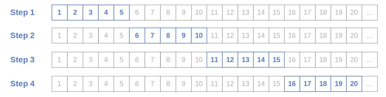
The name comes from the jumps of size $m$ between the steps. For instance, this is how the algorithm runs when $m=5$ :

3.1. Pseudocode

Here’s the pseudocode:

We can set $m$ to any value we like, but the algorithm’s complexity depends on our choice of $m$ .

3.2. Complexity Analysis

Let’s say that our list has $n$ elements. In the worst case, we check all the $\lceil \frac n m \rceil$ sub-lists’ boundaries and compare all the elements in the last sub-list to $z$ . So, we perform $O\left( \frac n m + m\right)$ comparisons.

The minimum of $\frac n m + m$ is $2 \sqrt{n}$ when $m = \sqrt{n}$ . So, if we set $\boldsymbol{m}$ to $\boldsymbol{\sqrt{n}}$ , Jump Search will run in $\boldsymbol{O(\sqrt{n})}$ time with respect to the number of comparisons.

However, to reach the new sub-list’s end, we need to follow $m$ pointers from the previous step’s $right$ . As a result, we traverse all $n$ nodes in the worst case. So, the algorithm has an $O(n)$ worst-case time complexity if we consider node traversals. However, if a comparison is more complex than following a pointer, we can say that the complexity is $O(\sqrt{n})$ .

3.3. Arrays

As we said before, Jump Search can handle arrays too. We prefer it over logarithmic Binary Search when going back (e.g., from testing if $\boldsymbol{x[n/2]=z}$ to checking whether $\boldsymbol{x[n/4]=z}$ ) is expensive or impossible.

That can happen when $x$ is so large that it can’t fit into the working memory or is a stream of data we’re downloading from an external source. In the former case, requesting $x[j/2]$ after $x[j]$ might require loading new blocks from the disk into RAM. In the latter case, downloading individual elements is expensive since we get them over a network, so going back and forth like in Binary Search would be slow.

4. Conclusion

In this article, we presented the Jump Search algorithm. We use it to search singly-linked lists in $O(\sqrt{n})$ time, but it can also search arrays.

Full Archive

About Baeldung

Core Concepts

Operating Systems

Artificial Intelligence

Graph Theory

Latex