Introduction to Graph Theory | Baeldung on Computer Science

1. Overview

In this tutorial, we’ll discuss some of the most important data structures in computer science – graphs.

We’ll first study the basics of graph theory, in order to familiarize ourselves with its conceptual foundation. We’ll then study the types of graphs that we can find in our machine learning applications.

At the end of this tutorial, we’ll know what a graph is and what types of graphs exist. We’ll also know what are the characteristics of the graph’s primitive components.

2. The Basics of Graph Theory

2.1. The Definition of a Graph

A graph is a structure that comprises a set of vertices and a set of edges. So in order to have a graph we need to define the elements of two sets: vertices and edges.

The vertices are the elementary units that a graph must have, in order for it to exist. It’s customary to impose on graphs the condition that they must have at least one vertex, but there’s no real theoretical reason why this is the case. Vertices are mathematical abstractions corresponding to objects associated with one another by some kind of criterion.

Edges instead are optional, in the sense that graphs with no edges can still be defined. An edge, if it exists, is a link or a connection between any two vertices of a graph, including a connection of a vertex to itself. The idea behind edges is that they indicate, if they are present, the existence of a relationship between two objects, that we imagine the edges to connect.

We usually indicate with $V = \{v_1, v_2, ... , v_n\}$ the set of vertices, and with $E = \{e_1, e_2, ... e_m\}$ the set of edges. We can then define a graph $G$ as the structure $G(V, E)$ which models the relationship between the two sets:

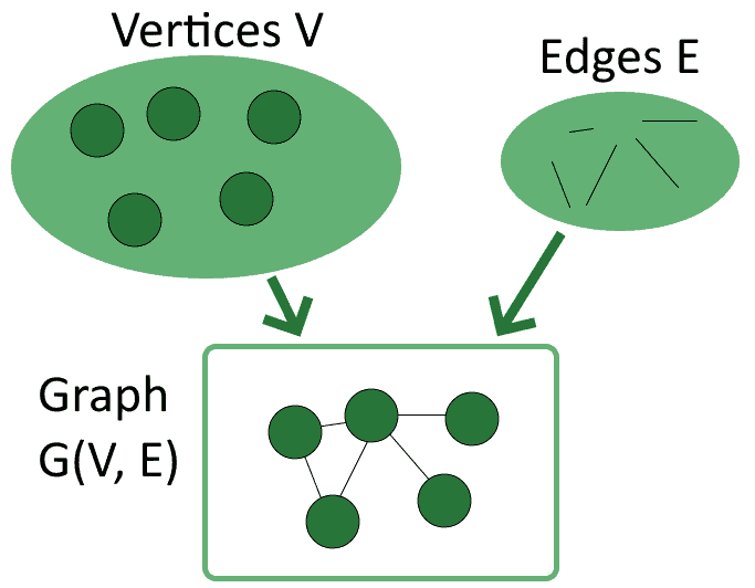
Notice how the order of the two sets between parentheses matters, because conventionally we always indicate first the vertices and then the edges. A graph $H(X, Y)$ is therefore a structure that models the relationship between the set of vertices $X$ and the set of edges $Y$ , not the other way around.

A brief note on terminology before we proceed further: graphs are a joint subject of study for both mathematics and network theory. The terms used in the two disciplines differ slightly, but they always refer to the same concepts. For this article, we’ll be using the terminology of mathematics, but we can use a conversion table to translate between the two if necessary.

2.2. General Properties of Vertices

We’re now going to focus in more detail about what characteristics vertices and edges possess. Let’s start with the vertices first.

As stated before, graphs need vertices but don’t necessarily require edges. In fact, it’s perfectly possible to have graphs $G(V, \O)$ composed entirely by vertices. Vertices that aren’t connected to any others, such as those of the empty graphs, are called isolated:

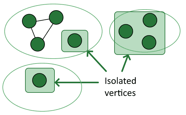
We also say that isolated vertices have a degree $\delta(v)$ equal to zero. Degree, in this context, indicates the number of incident edges to a vertex.

We say for vertices that aren’t isolated that they have a positive degree, which we normally indicate as $\delta(v)>0$ . The degree of a vertex can be any natural number.

The name leaf indicates a particular kind of vertex, one with degree $\delta(v) = 1$ . The term is in common with hierarchical trees, and similarly concerns vertices that are connected to one and only one other vertex.

2.3. Labels of Vertices

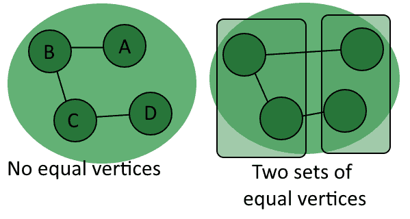
Vertices can also have values associated with them. These values can take any format and there are no specific restrictions for them. A vertex with an associated value is called a labeled vertex, while a vertex with no associated value is called unlabeled:

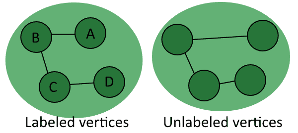
In general, we can distinguish any two unlabeled vertices exclusively on the basis of their paired vertices. The comparison between labeled vertices requires us instead to study both the pairs of vertices and the values assigned to them:

One final note on vertices concerns the number $|V|$ of them contained in a graph. This number has special importance, and we call it the order of the graph.

2.4. General Properties of Edges

We can now study the characteristics of edges. In contrast with vertices, edges can’t exist in isolation. This derives from the consideration that graphs themselves require vertices in order to exist, and that edges exist in relation to a graph.

An edge can connect any two vertices in a graph. The two vertices connected by an edge are called endpoints of that edge. By its definition, if an edge exists, then it has two endpoints.

Graphs whose edges connect more than two vertices also exist and are called hypergraphs. This tutorial doesn’t focus on them, but we have to mention their existence because of their historical and contemporary importance for the development of knowledge graphs.

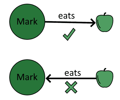
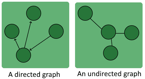
2.5. Endpoints, Directions, Loops

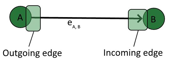
It’s possible to further distinguish between the two endpoints of an edge, according to whether they point towards a vertex or rather away from it. We call an edge going towards a vertex an incoming edge, while we call an edge originating from a vertex an outgoing edge:

In the image above, the edge $e_{A,B}$ connecting the pair $(A,B)$ is not reciprocated by a corresponding edge $e_{B,A}$ connecting $B$ to $A$ . In this case, we say that the graph $G(\{A, B\}, \{e_{A, B}\})$ is a directed graph, and we call the edge $e_{A, B}$ an arc.

Edges can also be undirected, and connect two vertices regardless of which one is the vertex of origin for that edge. Edges of this type are called lines and are such that any two vertices $(A, B)$ connected by them can be traversed in both directions. One way to look at this is to imagine that a line $e'$ between $A$ and $B$ corresponds to an arc $e_{A, B}$ plus an arc $e_{B, A}$ :

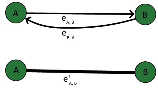
The advantage of this type of thinking is that it translates well to adjacency matrices of graphs.

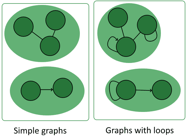
Furthermore, an edge can simultaneously be an incoming edge and an outgoing edge for the same vertex. In this case, we call that edge a loop.

Loops are a special kind of edge and aren’t present in all graphs. We call graphs without loops simple graphs, in order to distinguish them from the others:

Finally, we can mention that the number of edges $|E|$ in a graph is a special parameter of that graph. We call this number the size of the graph, and it has some special properties that we’ll see later.

2.4. Paths in a Graph

A graph with a non-empty set of edges has paths, which consist of sequences of edges that connect two vertices. We can call paths that relate to sequences of directed edges, unsurprisingly, directed paths; paths related to undirected edges however don’t have a special name.

One way to look at the relationship between paths and graphs is to imagine that each graph is a labyrinth and that each of its vertices is an intersection:

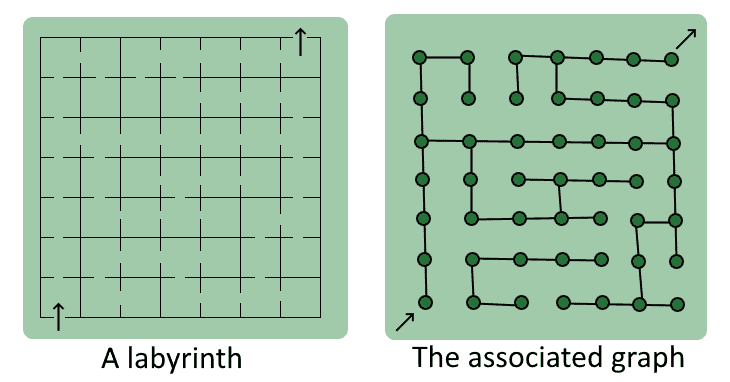
In this model, the starting vertex of a path corresponds to the entrance of the maze, and the target vertex corresponds to the exit. If we use this conceptual framework we can then imagine traversing the labyrinth and leaving a trail behind, which we then call a path.

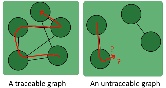
One special kind of path is the one that traverses all vertices in a graph, and that’s called a Hamiltonian path. Hamiltonian paths aren’t necessarily present in all graphs. We call graphs that contain Hamiltonian paths traceable because it’s possible to leave a full trace that covers all of their vertices:

Finally, we can mention that paths whose start and end vertices coincide are special, and are called cycles. It’s important to detect cycles in graphs because the algorithms for finding paths may end up looping over them indefinitely.

One last note on why paths are particularly important in computer science. This is because there are efficient algorithmic ways such as Dijkstra’s algorithm and A* that allow us to easily find the shortest paths. This, in turn, allows the computer resolution of problems such as the optimization of processes, logistics, and the processing of search queries.

3. Types of Graphs

3.1. The Empty Graph

We mentioned before that graphs exist only if their set of vertices is not null. Their set of edges, however, may as well be empty. If this is the case, we say that the graph is empty:

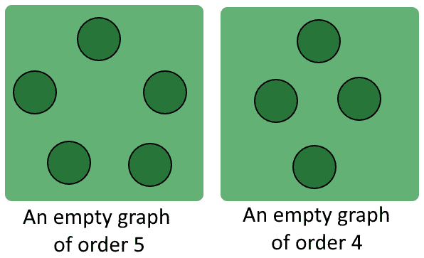
An empty graph $G(V, \O)$ has always size $|E| = 0$ .

3.2. The Directed Graph

As anticipated above, a directed graph is a graph that possesses at least one edge $e_{A, B}$ between two vertices $A$ and $B$ which doesn’t have a corresponding edge $e_{B, A}$ connecting the same vertices in the opposite direction.

Directed graphs have the characteristic that they model real-world relationships well for which we can’t freely interchange the subject and the object. As a general rule, if we aren’t sure whether a graph should be directed or undirected, then the graph is directed:

We can only traverse directed graphs in the directions of their existing directed edges.

Regarding directed graphs, we can briefly mention that there are general methods for determining whether a directed graph contains the maximum number of possible edges. This is important for reasons that have to do with the entropy of a directed graph.

3.3. The Undirected Graph

Undirected graphs are graphs for which the existence of any edge $e_{A, B}$ between the vertices $(A, B)$ implies the presence of a corresponding edge $e_{B, A}$ :

Undirected graphs allow their traversal between any two vertices connected by an edge. The same isn’t necessarily true for directed graphs.

3.4. The Connected and Disconnected Graphs

We can also discriminate graphs on the basis of the characteristics of their paths. For example, we can discriminate according to whether there are paths that connect all pairs of vertices, or whether there are pairs of vertices that don’t have any paths between them. We call a graph connected if there is at least one path between any two of its vertices:

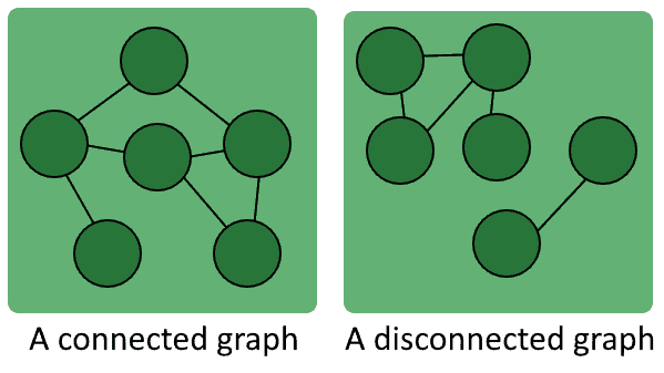
Similarly, we say that a graph is disconnected if there are at least two vertices separated from one another.

3.5. The Hamiltonian-Connected Graph

A Hamiltonian-connected graph is a graph for which there is a Hamiltonian path between any two of its vertices. Notice how connected graphs aren’t necessarily Hamiltonian-connected:

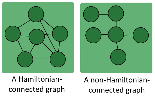
A Hamiltonian-connected graph is always a traceable graph, but the opposite isn’t necessarily true.

3.6. The Complete Graph

We say that a graph is complete if it contains an edge between all possible pairs of vertices. For a complete graph of order $|V|$ , its size $|E|$ is always $|E| = \frac{|V| \cdot (|V| - 1)}{2}$ :

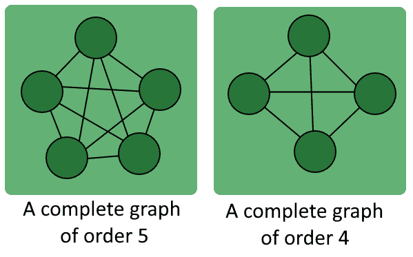
All complete graphs of the same order with unlabeled vertices are equivalent.

3.7. The Tournament

A tournament is a kind of complete graph that contains only directed edges:

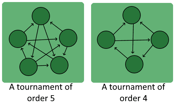
The name originates from its frequent application in the formulation of match composition for sports events.

3.8. The Weighted Graph

The final type of graph that we’ll see is a weighted graph. A weighted graph is a graph whose edges have a weight (that is, a numerical value) assigned to them:

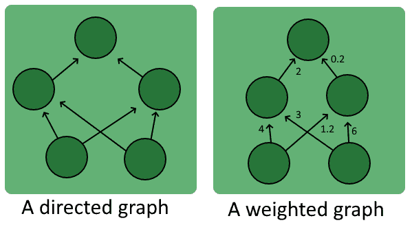
A typical weighted graph commonly used in machine learning is an artificial neural network. We can conceptualize neural networks as directed weighted graphs on which each vertex has an extra activation function assigned to it.

4. Conclusions

In this tutorial, we studied the conceptual bases of graph theory. We also familiarized ourselves with the definitions of graphs, vertices, edges, and paths.

We’ve also studied the types of graphs that we can encounter and what are their predictable characteristics in terms of vertices, edges, and paths.

Full Archive

About Baeldung

Core Concepts

Operating Systems

Artificial Intelligence

Graph Theory

Latex