Overview of Dijkstra’s Algorithm

1. Introduction

Many times in writing software, we need to be able to find the best route between two points in a graph. This is very commonly used in computer games, but also mapping software such as Google Maps, and can find uses in many other types of software as well.

Dijkstra’s Algorithm is a very popular pathfinding algorithm used for finding the shortest route between two points in the same graph.

2. What Is Pathfinding?

Pathfinding is an algorithm for graph traversal, where we have a start and end node and need to determine the best route between the two. This involves both the number of steps on the route, as well as the cost of each step.

This cost is dependent on the type of graph that we’re working with – a real-world map might be measured in meters, whereas a computer game like Civilization might base this on the type of unit that is moving and the type of terrain it’s moving over.

There are even applications of pathfinding for traversing state machines, where each node in the graph corresponds to a state, and each edge corresponds to a transition. This can then be used for finding the most efficient set of transitions between two states, like when solving a Rubik’s Cube.

3. Dijkstra’s Algorithm

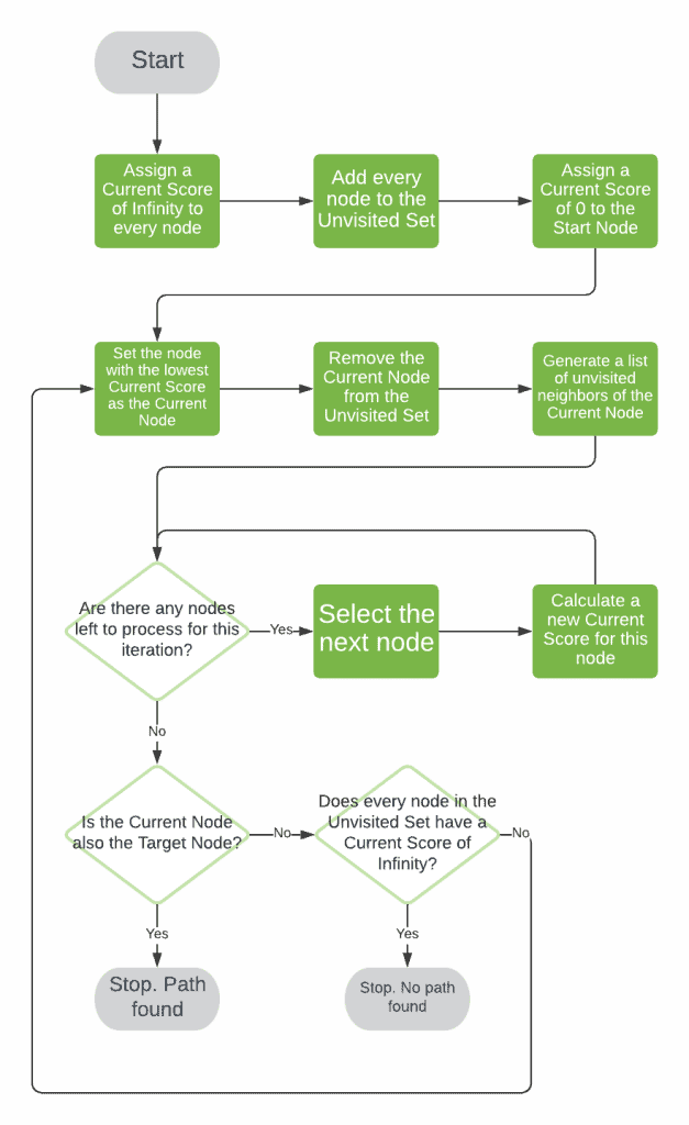
Dijkstra’s Algorithm is a pathfinding algorithm that generates every single route through the graph, and then selects the route that has the lowest overall cost.

This works by iteratively calculating a distance for each node in the graph, starting from the start node, and continuing until we reach the end node. In every iteration we have a “current node,” and we compute a new best score for every node that can be reached from it.

3.1. Flowchart

3.2. Pseudocode

Now that we know how the algorithm is going to work, what does it look like? Let’s explore some pseudocode describing the algorithm in more detail.

The core of the algorithm is an iterative process, looking at the current best node each time until we reach our target.

algorithm Dijkstra(graph, startNode, targetNode):
    // INPUT
    //     graph, startNode, targetNode
    // OUTPUT
    //     The shortest path from startNode to targetNode in the graph

    for each node in graph:
        node.score <- infinity
        node.visited <- false

    startNode.score <- 0

    while true:
        currentNode <- nodeWithLowestScore(graph)
        currentNode.visited <- true

        for nextNode in currentNode.neighbors:
            if nextNode.visited = false:
                newScore <- calculateScore(currentNode, nextNode)
                if newScore < nextNode.score:
                    nextNode.score <- newScore
                    nextNode.routeToNode <- currentNode

        if currentNode = targetNode:
            return buildPath(targetNode)

        if nodeWithLowestScore(graph).score = infinity:
            throw a NoPathFound exception

As a part of this, we need to be able to find the current best node. This is the node that has the lowest score that we’ve calculated so far, and that we’ve not already visited.

algorithm nodeWithLowestScore(graph):
    // INPUT
    //     graph = the input graph
    // OUTPUT
    //     The node with the lowest score that has not been visited

    result <- null
    for each node in graph:
        if node.visited = false and (result is null or node.score < result.score):
            result <- node

    return result

Next we need to calculate the new score for a node. This is the current score for the node that we’re coming from added to the edge cost of reaching the new node from it.

algorithm calculateScore(currentNode, nextNode):
    // INPUT
    //     currentNode, nextNode
    // OUTPUT
    //     score for moving from currentNode to nextNode

    return currentNode.score + currentNode.edgeCost(nextNode)

Finally, once we reach our target we then need to actually build our route. This is the list of nodes that we have to traverse to get from start to end. By recording on each node the best previous node, we’re effectively building this list as we go so we just need to pull it together.

algorithm buildPath(targetNode):
    // INPUT
    //     targetNode
    // OUTPUT
    //     The route from startNode to targetNode

    route <- create an empty list
    currentNode <- targetNode

    while currentNode != null:
        route.add(currentNode)
        currentNode <- currentNode.routeToNode

    return route

4. Conclusion

Here we’ve seen what pathfinding algorithms are in general, and what Dijkstra’s Algorithm is specifically. We’ve also seen how it works, so we can see how to apply this to our future problems.