Depth-First Search vs. Breadth-First Search | Baeldung on Computer Science

1. Introduction

In this tutorial, we’ll talk about Depth-First Search (DFS) and Breadth-First Search (BFS). Then, we’ll compare them and discuss in which scenarios we should use one instead of the other.

2. Search

Search problems are those in which our task is to find the optimal path between a start node and a goal node in a graph. There are several variations to search problems: the graph may be directed or undirected, weighted or unweighted, and there may be more than one goal node.

DFS and BFS are suitable for unweighted graphs, so we use them to find the shortest path between the start and the goal.

3. Depth-First Search and Breadth-First Search

Both algorithms search by superimposing a tree over the graph, which we call the search tree. DFS and BFS set its root to the start node and grow it by adding the successors of the tree’s current leaves. In that way, DFS and BFS cover the whole graph until they find the goal node or exhaust the graph. What they differ in is the order in which they visit the nodes, i.e., add them to the search tree.

In each step, DFS adds to the tree a child of the most recently included node with at least one unincluded child. So, DFS adds the start node, then its child, then its grandchild, and so on. For that reason, DFS increases the depth of the search tree in each step as much as it can. Then, if there aren’t more children of a node to add, it backtracks to the node’s parent.

In contrast, BFS grows the tree layer by layer. It first adds all the start node’s children, thus completing level 1. Then, it adds all the children of all the leaves at the first level one by one. Afterward, it adds all the children of the start node’s grandchildren, and so on. So, if the branching factor is constant across all the levels, BFS makes the tree wider at each step. To do so, BFS does the opposite of DFS: it adds to the tree a child of the least recently added node that has at least one unincluded child.

3.1. Tree-Like Search vs. Graph Search

Both algorithms may come in two variants: Tree-Like Search and Graph Search. The Tree-Like Search (TLS) versions don’t check for repeated nodes and may include the same node more than once in the tree. That is why they’re prone to get stuck in a loop. In contrast, the Graph-Search (GS) alternatives check for repetitions, so they’re immune to cycles but require more memory.

We’ll focus on the TLS versions since it’s easier to spot the differences between them.

4. Conceptual Difference

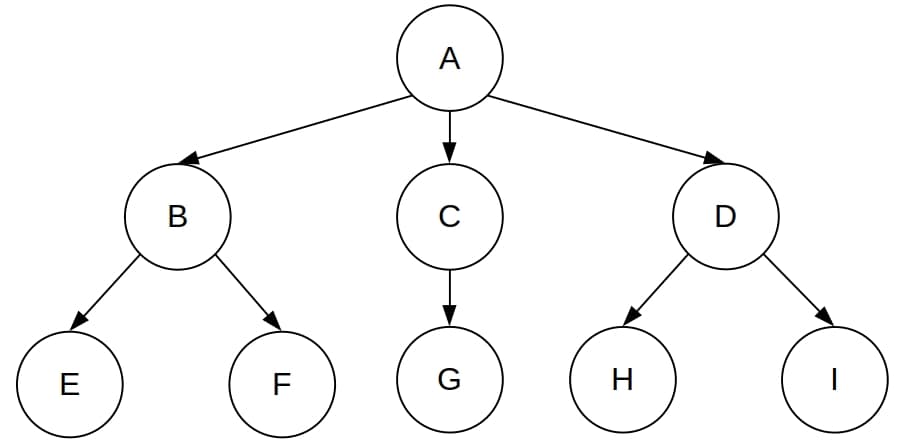
The following example illustrates the main conceptual difference between DFS and BFS. Let’s imagine that we’ve got the following search tree:

Let’s mark each node by the ordinal number of its inclusion in the tree. The orders in which DFS and BFS include the nodes differ:

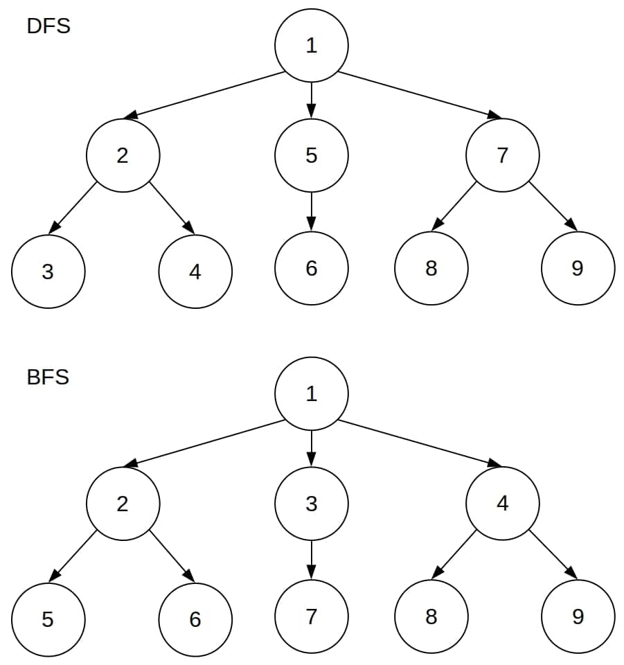
In the BFS tree, all the inclusion numbers at level $i$ are lower than the numbers at level $i+1$ . That’s not the case in DFS. In DFS, if node $u$ has a lower inclusion number than node $v$ , then all the descendants of $u$ have lower numbers than $v$ and its descendants.

So, BFS grows the tree level by level, whereas DFS grows it sub-tree by sub-tree.

5. Implementation Differences

At each execution step, both DFS and BFS maintain what we call the search frontier. It’s a set of nodes we identified as children of the nodes currently in the tree but didn’t add to it yet. Since BFS always adds the child of the least recently included node, it uses a FIFO queue to maintain the frontier. In contrast, DFS uses a LIFO queue in its iterative implementation.

When adding a node to the search tree, we also identify its children and add them to the frontier. That’s called expanding the node. So, we can describe BFS and DFS as follows:

DFS expands the deepest node in the frontier.
BFS expands the shallowest node.

DFS is also very suitable for a recursive implementation. In that case, the call stack acts as a frontier.

6. Differences in Completeness and Optimality

We say that a search algorithm is complete if it always terminates. That means that the algorithm finds a path to the goal if at least one goal is reachable from the start. Otherwise, it returns a notification of failure.

If an algorithm returns the optimal path to a goal node, provided that at least one is present in the graph, we say that the algorithm is optimal.

6.1. Completeness

DFS isn’t a complete algorithm. To see why let’s imagine that the graph contains a cycle $u{-}v{-}w{-}u$ . Depending on the choice of the successor to add first to the tree when considering the successors of a node, DFS may get stuck in a loop:

$u{-}v{-}w{-}u{-}v{-}w{-}u{-}v{-}w{-}u{-}v{-}w{-}u{-}v{-}w{-}u{-}v{-}w{-}u{-}v{-}w{-}u\ldots$

Even if we randomize the choice, we can still end in a loop and run indefinitely, although such an outcome is less likely. So, DFS may never terminate even if the goal is very close to the start node and the graph is finite and small:

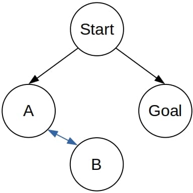
If (the TLS version of) DFS goes to $A$ , it will forever alternate between $A$ and $B$ .

On the other hand, BFS is always complete if the graph is finite. If the graph is infinite, then BFS is complete under the following condition:

A goal node is reachable from the start, and no node has an infinite number of successors.

6.2. Optimality

DFS isn’t an optimal algorithm either. It may return a sub-optimal path to the goal, and that happens if the goal is reachable in more than one way, but DFS discovers a longer path first:

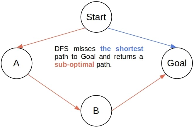
In contrast, BFS is optimal.

7. Complexity Differences

Before we analyze complexity, let’s introduce the notation. Let $b$ be the tree’s branching factor, $m$ the length of the longest path in the graph, and $d$ the depth of the shallowest goal node. If no goal is reachable from the start, we’ll consider that $d=m$ . Also, we’ll consider only the cases where the algorithms terminate.

7.1. Time Complexity

In the worst-case scenario, DFS creates a search tree whose depth is $m$ , so its time complexity is $O(b^m)$ .

Since BFS is optimal, its worst-case outcome is to find the goal node after adding $b$ nodes at level 1, $b^2$ at level 2, and so on up to level $d$ where it adds $b^d$ nodes. In total, the worst-case tree of BFS contains $1+b+b^2+\ldots+b^d$ nodes, which means that the time to grow it is of the order $O(b^d)$ .

7.2. Space Complexity

Since BFS keeps adding more nodes to the frontier but pops the oldest among them, it has to store all of them. So, its space complexity in the worst-case scenario is $\boldsymbol{O(b^d)}$ because that’s the worst-case size of the frontier.

DFS is different. After exploring the whole subtree whose root is node $u$ , DFS tries the siblings of $u$ . But, while processing $u$ and its descendants, DFS doesn’t have to keep the descendants of the $u$ ‘s siblings in the main memory. It can focus only on the currently active path, and all it needs for backtracking are the siblings of the nodes on it. So, the worst-case space complexity of DFS is $\boldsymbol{O(bd)}$ .

We can reduce the complexity of DFS if we yield the children of the deepest node on the currently active path one by one instead of returning them all at once. In that case, we store no more than $d$ nodes at any point during execution. And we can go even further! If we can transform the nodes to one another, we can use a single node and apply transformations when replacing it with its child or siblings. As a result, we get an $O(1)$ space complexity, but the transformations have to be reversible because of backtracking.

8. How to Choose Between DFS and BFS?

All this said, the actual question we’re interested in is how to choose between DFS and BFS.

If we know that the goal is deep, we should use DFS because it reaches deep nodes faster than BFS. A good example is constraint satisfaction. In those problems, we have to assign values to several variables such that the constraints on the variables and their values are satisfied. Each node in the resulting search graph is a list of assignments. Since we’re interested in complete solutions, it makes more sense to reach the full assignment nodes as fast as possible with DFS than to slowly search through incomplete assignments with BFS.

On the other hand, if we know that the goal may appear at a shallow level in the search tree, BFS is a better choice. The same goes if we cannot accept a sub-optimal path and are ready to spend more memory to get the theoretical guarantees. But, the caveat is that BFS can require a lot of memory and will prove inefficient if the branching factor is too large or the goal is deep.

It’s precisely the memory complexity that makes BFS impractical even though it’s complete and optimal in the cases where DFS isn’t. For that reason, DFS has become the working horse of AI. We can even sort out the problems of its incompleteness and sub-optimal solutions. Iterative deepening, which limits the depth of DFS and runs it with incremental limiting depths, is complete, optimal, and of the same time complexity as BFS. However, its memory complexity is the same as that of DFS.

8. Conclusion

In this article, we compared Depth-First Search (DFS) to Breadth-First Search (BFS). While BFS has some theoretical advantages over DFS, it’s impractical because of the high order of its space complexity. That is why we use DFS more often.

Full Archive

About Baeldung

Core Concepts

Operating Systems

Artificial Intelligence

Graph Theory

Latex