From Recursive to Iterative Functions

1. Introduction

In this tutorial, we’ll talk about ways to convert a recursive function to its iterative form. We’ll present conversion methods suitable for tail and head recursions, as well as a general technique that can convert any recursion into an iterative algorithm.

2. Recursion

Recursion offers many benefits. Many problems have a recursive structure and can be broken down into smaller sub-problems. So, solving the sub-problems recursively and combining their solutions is a natural way to handle such problems. For that reason, recursive functions are easier to read, understand, and maintain.

However, recursion doesn’t come without issues of its own. Because each recursive call adds a new frame to the call stack, recursive functions may run out of stack memory if dealing with very large inputs, causing the stack overflow error. Additionally, recursive functions may be of higher memory and space complexity than their iterative counterparts. Let’s take a look at the recursive and iterative functions for computing the Fibonacci numbers:

The recursive function is more readable because it follows the definition of Fibonacci numbers:

However, since the stack’s depth is limited, it will throw an overflow for large . In contrast, the iterative function runs in the same frame. Moreover, the recursive function is of exponential time complexity, whereas the iterative one is linear. That’s why we sometimes need to convert recursive algorithms to iterative ones. What we lose in readability, we gain in performance.

3. Converting Tail-Recursive Functions

The most straightforward case to handle is tail recursion. Such functions complete all the work in their body (the non-base branch) by the time the recursive call finishes, so there’s nothing else to do at that point but to return its value. In general, they follow the same pattern:

The accumulator is the variable that holds partial solutions during execution. They represent the solutions to a sequence of sub-problems, nested one within the other. Each call updates the accumulator until the recursion reaches the base case. At that point, the accumulator holds the solution to the entire problem we started solving in the beginning.

3.1. Iterative Version of Tail Recursion

The above pattern of tail recursion has the following iterative version:

From this, we formulate the general rules of conversion:

• Initialize the accumulator before the while-loop.
• Use the negation of the base-case condition as the loop’s condition.
• Use the recursive function’s body (except the recursive call) as the body of the while-loop.
• After the loop, apply the base-case update of the accumulator and return its value.

Usually, the base-case update doesn’t change the accumulator’s value since it often amounts to a neutral operation such as adding 0 or multiplying by 1, or there’s no update to apply. So, we can ignore this part in most cases. Still, we keep it in the pseudo-code to account for the functions whose base-case update is non-trivial. For example, that’s the case if we have multiple base cases, and each combines a different value with the accumulator. It’s also the case if the base-case update depends on the accumulator.

3.2. Example

Let’s put those rules to use and convert a tail-recursive function for calculating factorials:

Let’s now identify the elements of this tail recursion that we’ll reorder in the iterative variant:

• base-case condition:
• base-case accumulator update: multiply by 1
• the initial value of the accumulator: 1
• the accumulator update:
• problem reduction: from to

With that in mind, we get the following iterative function:

Even though the negation of is instead of , we use the latter because is restricted to natural numbers.

4. General Conversion Method

We saw how we could turn tail-recursive functions to be iterative. However, there are other recursion types. For example, a head-recursive function places the recursive call at the beginning of its body instead of its end. Other types surround the call with the code blocks for pre-processing the input and post-processing the call’s return value. What’s more, a recursive function can make any number of recursive calls in its body, not just one.

Luckily for us, there’s a general way to transform any recursion into an iterative algorithm. The method is based on the observation that recursive functions are executed by pushing frames onto the call stack and popping them from it. Therefore, if we simulate our stack, we can execute any recursive function iteratively in a single main loop. The resulting code, however, may not be pretty. That’s why we usually first try to make our function tail-recursive. If we succeed, we can get fairly readable code using the method from Section 3. If not, we use the general conversion method. So let’s first inspect the general form of recursive functions.

4.1. General Form of Recursion

A  recursive function can make an arbitrary number of recursive calls in its body:

This pseudo-code covers the cases where the number of recursive calls () is constant or bounded, like in binary-tree traversal (), as well as those where depends on the problem’s size. Also, a base-case solution can be constant or depend on that passes the test. Furthermore, each non-recursive code blocks can be empty or a single instruction or include calls to other subroutines. The purpose of is to prepare the data for the -th recursive call. Finally, combining recursive sub-solutions should also be understood generally: it can be as simple as or more complex.

4.2. The Execution Graph

Each call to creates a frame. It’s a structure holding the passed parameters, local variables, and the placeholder for the return value. If we visualized the frames and tracked the calls, we’d see that the recursive function defines an implicit and directed graph. Its nodes are frames, some of which have no out-looking edges. They represent the base cases of our recursion. Others have inward and outward edges: they model the calls between the base cases and the first call. Let’s see a portion of the graph for the Fibonacci numbers:

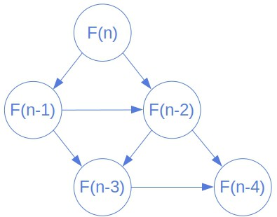
A directed edge from to corresponds to a recursive call in that makes the active frame. Accordingly, executing a recursive function is the same as traversing the frame graph in a structured way. We cross over each edge twice: the first time when makes the call that creates the ‘s frame and the second time when returns the call’s value to .

4.3. Execution as Depth-First Traversal

So, we start in the original caller’s frame node and execute the non-recursive code block before the first recursive call. At that point, we’ve created a child node that represents the call’s frame. The way recursion works implies that we should move to the child node and visit its descendants in the same manner. Afterward, we collect its frame’s return value, go back to the start node, and move to the next child. The goal is to visit all the nodes and return to the initial frame, at which point we combine the children’s return value and output the solution.

But, how does this graph help us turn a recursive function into an iterative one? The answer lies in the fact that we’ve just described a depth-first traversal of the execution graph. The iterative version of depth-first traversal uses a stack to store the nodes marked for visiting. If we implement the nodes and edges in a way that corresponds to the elements of our function, we’ll get its iterative version. There, the stack for storing the nodes plays the role of the call stack of a CPU:

4.4. Implementation Details

The execution graph is implicit. That means that we create it on the fly as we execute non-recursive code blocks and make recursive calls. To do it properly, we should implement the frames and edges following the structure of the recursive function we’re transforming.

So, should return the edge associated with the first non-executed NRCB and recursive call. It should also contain the pointer to the child frame we get by following the edge. So, this function should divide the problem into sub-problems and create child frames. A-frame should be a data structure capable of holding its local variables and its sub-problem. It should also be able to pass its return value to its parent.

is responsible for determining the value. If the frame is a base-case node, then the function should return the appropriate base-case solution. If not, then the function should combine the return values that the frame got from its children.

4.5. Example

Let’s convert this recursion into iteration:

4.6. Frames, Edges, and Edge Creation

In our example, could be a Python dictionary we’d create like this:

def create_new_frame(n, parent, return_name):
    # create an empty frame
    frame = {
        'n' : None,
        'parent' : None,      # the parent frame
        'return_name' : None, # the return address
        'placeholders': {     # the placeholders for 
            'a' : None,   # the children's return values
            'c' : None
        },
        'local': {            # the local variables 
            'b' : None,
            'd' : None
        },
    }

    # fill in the fields
    frame['n'] = n 
    frame['parent'] = parent 
    frame['return_name'] = return_name
    return frame

An instance of Frame should be coupled with functions to calculate the return value and pass it to the frame’s parent:

def get_return_value(frame):
    if frame['n'] <= 1:
        # the base case
        return 1
    else:
        # the recursive case
        frame['local']['d'] = frame['placeholders']['a'] * frame['placeholders']['c']
        return frame['local']['d'] + 1

def pass_to_parent(frame, return_value):
    return_name = frame['return_name']
    frame['parent']['placeholders'][return_name] = return_value

In this implementation, we don’t need to model edges. From Algorithm 7, we see that an edge should contain a child frame (the node it’s directed to) and the corresponding NRCB. We can model an NRCB as an integer that we’d include as another integer field, nrcb_counter, into the frames, initialize to 0 in create_new_frame, and interpret with the following function:

def execute_nrcb(frame):
    nrcb_counter = frame['nrcb_counter']
    if nrcb_counter == 1:
        # do nothing because the NRCB
        # before the first call (f(n-1))
        # is empty
        pass
    elif nrcb_counter == 2:
        frame['local']['b'] = frame['n'] // 2	

We’ll update the counter and execute the corresponding NRCB in the function that returns the next child frame:

def get_next_child(frame):
    # check if all the frame's NRCBs have been executed
    if frame['nrcb_counter'] >= 2:
        return None
    frame['nrcb_counter'] += 1
    execute_nrcb(frame)
    if frame['nrcb_counter'] == 1:
        child = create_new_frame(frame['n'] - 1, frame, 'a')
    else:
        child = create_new_frame(frame['placeholders']['b'], frame, 'c')
    return child

We test if frame has an unvisited out-going edge by verifying that it’s not a base-case frame and checking if frame.nrcb_counter < 2. The whole code would look like this:

def has_next_child(frame):
    return frame['n'] > 1 and frame['nrcb_counter'] < 2

def solve(n):
    start = create_new_frame(n, None, None)
    stack = [start]
    while len(stack) > 0:
        frame = stack.pop(-1)
        if has_next_child(frame):
            child = get_next_child(frame)
            stack.append(frame)
            stack.append(child)
        else:
            return_value = get_return_value(frame)
        if frame['parent'] is not None:
            pass_to_parent(frame, return_value)
    return get_return_value(start)

4.7. Readability and Semantics

Supplying the general depth-first traversal algorithm with recursion-specific implementations of the frames, edges, and associated functions, we get an iterative variant of the recursive function we wanted to transform. However, the resulting iterative code will not be as readable and understandable as the original recursive one.

We do retain some semantics in the graph, though. Because it embodies the recursive structure of the original problem, we can still interpret it. A node with its children represents the body of recursion, while the base case can be recognized in the nodes with no children.

4.8. Optimization and Types of Recursion

Finally, we note that we can visit some nodes in the graph more than once. That’s the case if sub-problems overlap, as is the case with the Fibonacci numbers. Both and depend on , so would be visited twice. Multiple visits to the same node result in repeated calculation and increased complexity. We can address this issue by remembering the return values. Whenever we compute the value a node should return, we store it in the node. If we later visit the same node, we reuse the solution already found and avoid repeated evaluation. This technique is called memoization. Some authors consider it a tool of dynamic programming.

Further, the shape of the execution graph reveals the difference between various recursion types. The graph of a recursive function that makes only one recursive call in its body is a path. If it makes two calls and the sub-problems don’t overlap, the resulting graph will be a binary tree. Tail recursion is specific because its recombination phase is an identity operation: each node only forwards the child’s return value. That’s why we don’t need a stack to make it iterative.

5. Why Convert Recursion to Iteration

Recursion and iteration are equally powerful. Any recursive algorithm can be rewritten to use loops instead. The opposite is also true. This means that any iterative algorithm can be written in terms of recursion only. Thus, if we have to choose one to use, our decision is likely to come down based on these issues:

• Expressiveness: we choose the method that makes the code simpler (thus reducing the opportunities for making mistakes). That is to reduce the time spent testing and debugging code
• Performance: iteration is usually (though not always) faster than an equivalent recursion. In addition, the time complexity of iteration is generally polynomial-logarithmic, while it’s generally exponential with a recursion algorithm

Furthermore, several popular programming languages do not support recursion. When trying to drop a large input into a recursive algorithm (for example, Python), we’ll almost certainly reach the runtime’s recursion limit. This refers to how many times the function can call itself so that infinite recursions are avoided.

Recursive functions require a lot of memory. Each recursion doubles the amount of memory allocated by the function, and the data is stored on a stack. A stack has a limited amount of memory, and if this limit is reached, then we’ll run out of stack space and the program can no longer run.

Therefore, knowing how to convert recursive algorithms into iterative algorithms is an important skill.

6. Advantage of Converting Recursion to Iteration

Converting a recursive function to an iterative function can have several advantages. Let’s discover some of them:

• Improved memory efficiency: iterative functions use a single stack frame, making them more memory-efficient compared to recursive functions which create a new stack frame for each recursive call
• Increased performance: iterative functions can be faster than recursive functions because they avoid the overhead of creating and destroying stack frames for each recursive call
• Easier to understand and maintain: converting a tail-recursive function to an iterative function can make the code easier to understand and maintain by removing the recursive calls

7. Conclusion

In this article, we talked about converting recursion into iteration. We presented a general way to transform any recursive function into an iterative one. Also, we showed a method for tail recursion only. Even though conversion may give us gains in performance, the code loses readability this way.