How to Find Common Elements in Two Sorted Arrays

1. Introduction

In this tutorial, we’ll explain how to find common elements in two sorted arrays.

2. Common Elements of Two Sorted Arrays

In this problem, we have two sorted arrays: $a=[a_1 \leq a_2 \leq \ldots \leq a_n]$ and $b=[b_1 \leq b_2 \leq \ldots \leq b_m]$ . Our task is to find the common elements.

For instance, if $a = [1, 2, 3, 4, 5]$ and $b = [3, 4, 5, 6, 7]$ , our algorithm should output $[3, 4, 5]$ as the result.

To find the common elements efficiently, it should use the fact that $a$ and $b$ are already sorted. Additionally, we’ll also require the output array to be non-descending as the input arrays.

We’ll also assume that $a$ and $b$ can contain duplicates. So, if a common element is repeated twice in $a$ , and thrice in $b$ , we’ll include it twice in the result array. For instance:

$\begin{equation*} \begin{matrix} a&=& [1& 2& 2& 4& 5] \\ b&=& [2& 2& 2& 3& 5& 7] \\ result&=& [2& 2& 5]\\ \end{matrix} \end{equation*}$

3. Finding Common Elements in Linear Time

Let’s start with the naive algorithm that doesn’t use the fact that $a$ and $b$ are sorted:

For each $a_i$ , the algorithm iterates over the entire $b$ to check if $a_i \in b$ . So, it has an $O(mn)$ time complexity, which implies $O(n^2)$ if $m$ and $n$ are comparable. What can we change in this algorithm to get common elements faster?

3.1. Linear Search

Well, since the arrays are sorted, there’s no point in iterating over $\boldsymbol{b_{j+1}, b_{j+2}, \ldots, b_{m}}$ if $\boldsymbol{a_i < b_j}$ . Each of those is greater than $a_i$ , so we can conclude that $a_i \not \in b$ . The converse is also true: if $b_j < a_i$ , we can discard $b_j$ .

That way, we iterate over each array only once. So, we don’t need nested loops. Instead, we can start with $i=1$ and $j=1$ . When $a_i < b_j$ , we discard $a_i$ by incrementing $i$ . Similar goes for $j$ if $b_j < a_i$ . If $a_i=b_j$ , we append $a_i$ to the result array and update both counters. The loop stops once we reach the end of $a$ or $b$ . This approach is similar to the merge step in the Merge Sort algorithm:

As a result, the algorithm’s time complexity is linear: $O(m + n)$ .

3.2. Example

Let’s use the above example to show how the algorithm works.

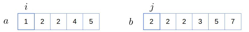
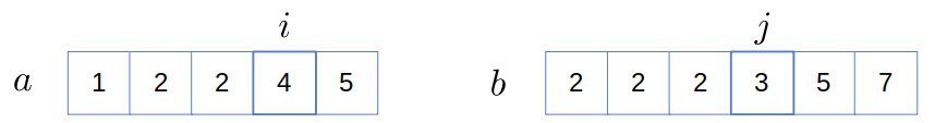
Initially, $c$ is empty, and both $i$ and $j$ point to the first elements:

Since $a_1=1 < a_2=2$ , we increment $i$ :

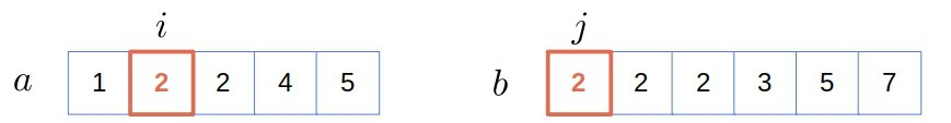
Now, we have a match, so we append 2 to $c$ and increment both counters:

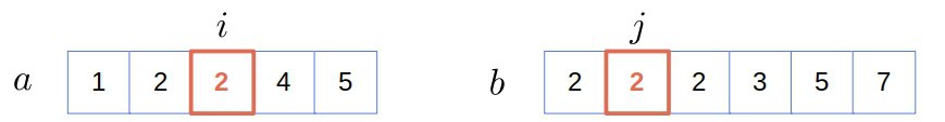
We have a match again, so we do the same as in the previous step:

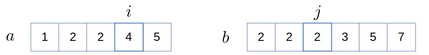
Now, $a_3=4 > b_3=2$ , so we discard $b_3$ and move on to $b_4$ :

The situation is the same ( $a_3=4 > b_4=3$ ), so we increment only $j$ :

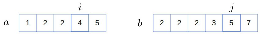
Since $a_3=4 < b_5 = 5$ , we increment only $i$ :

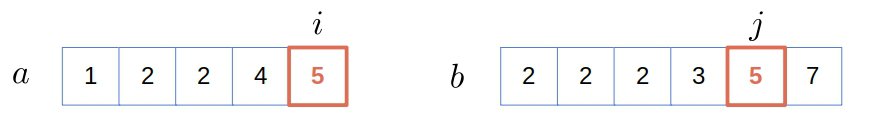
We found a new common element, so we add it to $c$ and increment both counters:

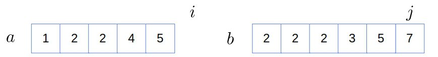
Finally, $i>n=5$ , so we stop and output the result: $c=[2, 2, 5]$ .

4. Finding Common Elements in Logarithmic Time

Let’s suppose that $m << n$ . Then, for each $\boldsymbol{j=1,2,\ldots,m}$ , we can look for $\boldsymbol{b_j}$ in $\boldsymbol{a}$ with the logarithmic binary search. Since $b_j \leq b_{j+1}$ , if the binary search finds $b_j$ at the $k$ -th position in $a$ , we can discard all the element to the left and search for $b_{j+1}$ in the remainder: $[a_{k+1}, a_{k+2}, \ldots, a_n]$ .

Similarly, let’s say the binary search doesn’t find $b_j$ in $a$ , but the last index it checks in $a$ is $k$ . If $b_{j+1} = b_j$ , we search for $b_{j+1}$ in $[a_{k+1}, a_{k+2}, \ldots, a_{n}]$ . On the other hand, if $b_{j+1} > b_j$ , it can still happen that $b_{j+1}=a_{k}$ , so we don’t discard $a_k$ .

4.1. Pseudocode

Here’s how the above algorithm works:

The worst-case time complexity is $O(m\log n)$ . If $m << n$ , we can consider $m$ to be a constant with respect to $n$ . In that case, the algorithm has an approximate $\boldsymbol{O(\log n)}$ complexity. However, if $m \in \Theta(n)$ , we get an $O(n \log n)$ algorithm. That’s still better than the naive approach but worse than the $O(n+m)$ runtime of the two-side linear search.

5. Conclusion

In this article, we presented two efficient ways of finding common elements of two sorted arrays. One approach has an $O(n+m)$ complexity, whereas the other combines binary and linear searches and runs in an $O(m \log n)$ time.

Full Archive

About Baeldung

Core Concepts

Operating Systems

Artificial Intelligence

Graph Theory

Latex