

1. Introduction
2048 is an exciting tile-shifting game, where we move tiles around to combine them, aiming for increasingly larger tile values.
In this tutorial, we’re going to investigate an algorithm to play 2048, one that will help decide the best moves to make at each step to get the best score.
2. How to Play 2048
A game of 2048 is played on a 4×4 board. Each position on the board may be empty or may contain a tile, and each tile will have a number on it.
When we start, the board will have two tiles in random locations, each of which either has a “2” or a “4” on it – each has an independent 10% chance of being a “4”, or otherwise a is a “2”.
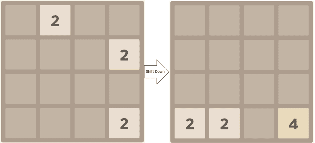
Moves are performed by shifting all tiles towards one edge – up, down, left, or right. When doing this, any tiles with the same value that are adjacent to each other and are moving together will merge and end up with a new tile equal to the sum of the earlier two:
After we’ve made a move, a new tile will be placed onto the board. This is placed in a random location, and will be a “2” or a “4” in the same way as the initial tiles – “2” 90% of the time and “4” 10% of the time.
The game then continues until there are no more moves possible.
In general, the goal of the game is to reach a single tile with a value of “2048”. However, the game doesn’t stop here, and we can continue playing as far as it is possible to go, aiming for the largest possible tile. In theory, this is a tile with the value “131,072”.
3. Problem Explanation
Solving this game is an interesting problem because it has a random component. It’s impossible to correctly predict not only where each new tile will be placed, but whether it will be a “2” or a “4”.
As such, it is impossible to have an algorithm that will correctly solve the puzzle every time. The best that we can do is determine what is likely to be the best move at each stage and play the probability game.
At any point, there are only four possible moves that we can make. Sometimes, some of these moves have no impact on the board and are thus not worth making – for example, in the above board a move of “Down” will have no impact since all of the tiles are already on the bottom edge.
The challenge is then to determine which of these four moves is going to be the one that has the best long-term outcome.
Our algorithm is based on the Expectimax algorithm, which is itself a variation of the Minimax algorithm, but where the possible routes through our tree are weighted by the probability that they will happen.
Essentially, we treat the game as a two-player game:
- Player One – the human player – can shift the board in one of four directions
- Player Two – the computer player – can place a tile into an empty location on the board
Based on this, we can generate a tree of outcomes from each move, weighted by the probability of each move happening. This can then give us the details needed to determine which human move is likely to give the best outcome.
3.1. Flowchart of Gameplay
The general flow of how the gameplay works:
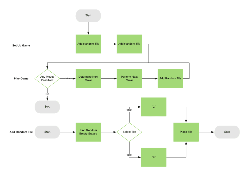
We can immediately see the random aspect of the game in the “Add Random Tile” process – both in the fact that we’re finding a random square to add the tile to, and we’re selecting a random value for the tile.
Our challenge is then to decide what to do in the “Determine Next Move” step. This is our algorithm to play the game.
The general overflow of this seems deceptively simple:
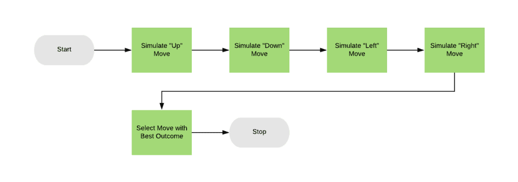
All we need to do is simulate each of the possible moves, determine which one gives the best outcome, and then use that.
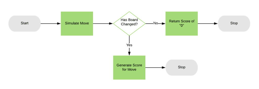
So we have now reduced our algorithm into simulating any given move and generating some score for the outcome.
This is a two-part process. The first pass is to see if the move is even possible, and if not, then abort early with a score of “0”. If the move is possible, then we’ll move on to the real algorithm where we determine how good a move this is:
3.2. Determining the Next Move
The key part of our algorithm so far is in simulating a move, and the key part of that is how we generate a score for each possible move. This is where our Expectimax algorithm comes in.
We’ll simulate every possible move from both players for several steps, and see which of those gives the best outcome. For the human player, this means each of the “up”, “down”, “left,” and “right” moves.
For the computer player, this means placing both a “2” or a “4” tile into every possible empty location:
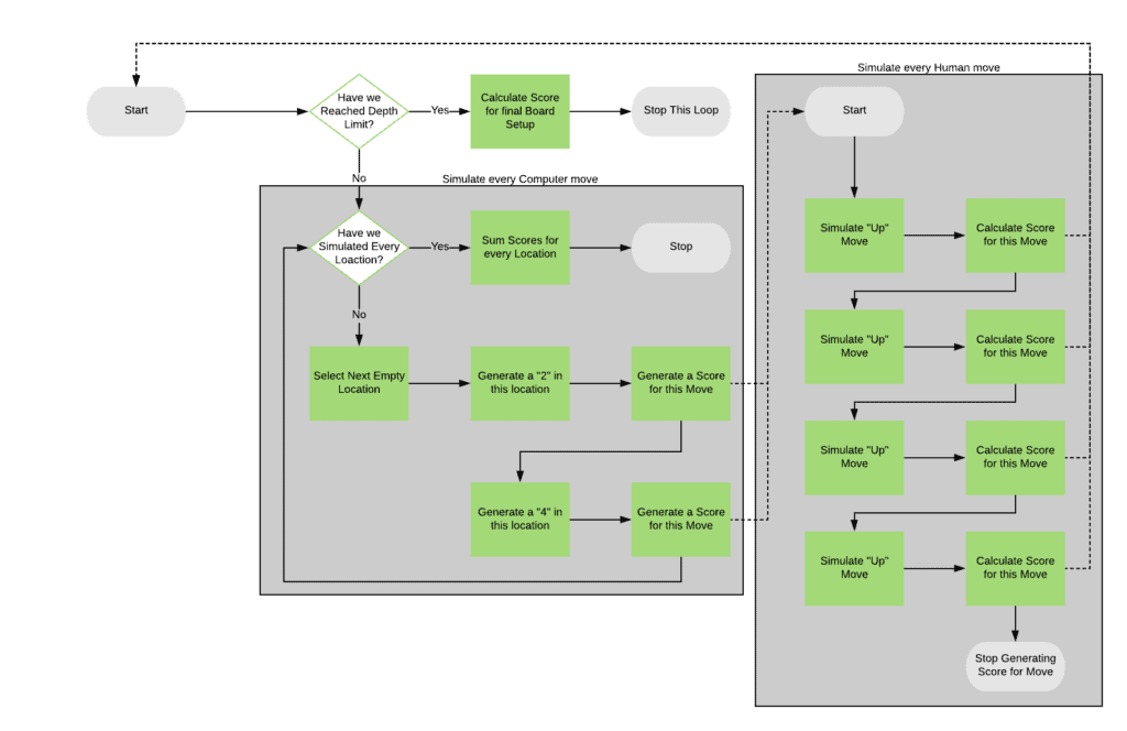
This algorithm is recursive, with each recursive step stopping only if it’s a certain depth from the actual move in the real game. That makes the flowchart harder to follow because it loops back on itself, but essentially we’ll:
- Stop if we’re at the depth limit, calculating a score for the currently simulated board layout
- Simulate every possible computer move
- For each of these
- Simulate every possible human move
- For each of these
- Recurse back into the algorithm
- Return the score calculated from this human move
- Add the score calculated from this computer move, weighted by a probability of this move happening
When we’ve finished this, we then add up all of the calculated scores, and this is the final score for the move we want to make from the current game board. Because we do this four times – one for each possible move from the current game board – we end up with four scores, and the highest of those is the move to make.
3.3. Scoring a Board Position
At this point, the only thing left to do is calculate a score for a board. This is not the same scoring as the game uses, but it needs to take into account how good a position this is to continue playing from.
There are a large number of ways that this can be achieved by adding several factors together with appropriate weightings. For example:
- Number of empty locations
- Number of possible merges – i.e., number of times the same number is in two adjacent locations
- The largest value in any location
- Sum of all locations
- Monotonicity of the board – this is how well the board is structured, such that location values increase in a single direction.
4. Pseudocode
Now that we know how the algorithm is going to work, what does this look like? Let’s explore some pseudocode describing the algorithm in more detail.
We’re not interested in the actual playing of the game, just in the algorithm for determining moves, so lets start there:

As before, this gets us to the point where we are simulating each of the possible moves from the starting board and returning the one that scores the best. This leaves us with needing to generate scores for the newly simulated boards.
We’ve added in a depth limit so that we can stop the processing after a while. Because we are working with a recursive algorithm, we need a way to stop it otherwise it will potentially run forever:


This gives us our recursion, simulating out every possible human and computer move for a certain number of steps and deciding which human moves give the best possible outcome.
The only thing left is to work out a final score for any given board position. There is no perfect algorithm for this, and different factors will give different results.

5. Performance Optimization
So far we’ve got an algorithm that will attempt to solve the game, but it’s not as efficient as it could be. Because of the random nature of the game, it’s impossible to have a perfectly optimized solver – there is always going to be some level of repetition simply because of the nature of the process.
We can at least do our best to reduce work that we don’t need to do though.
We’re already doing a bit of optimization in the above algorithm by not processing any moves that don’t have any impact on the game. There are other ways that we can reduce the work to do, though, such as tracking the cumulative probability of moves, and stopping when that gets too low. This does have the risk of removing the perfect solution, but if the probability is that low, then it almost certainly won’t happen anyway.
We can also dynamically determine the depth limit to work with. Our above pseudocode has a hard-coded limit of 3, but we could dynamically calculate this based on the shape of the board at the start of our calculations – for example, setting it to the number of empty squares or the number of distinct tiles on the board. This would mean that we traverse fewer moves from boards that have less scope for expansion.
Additionally, because it is possible to revisit the same board positions multiple times, we can remember these and cache the score for those positions instead of re-computing them every time. Potentially we can generate every possible board position ahead of time, but there are a huge number of these – 281,474,976,710,656 different possible board positions using tiles up to 2048 – so this is probably not feasible.
However, the most important optimization we can do is in adjusting the algorithm for generating board scores. This works to decide how good board is for continuing to play and the factors and weightings that we use for this are directly linked to how well our algorithm plays out.
6. Conclusion
2048 is a hugely interesting game to attempt to solve. There is no perfect way to solve it, but we can write heuristics that will search for the best possible routes through the game.
The same general principles work for any two-player game – for example, chess – where you can not predict what the other player will do with any degree of certainty.
Why not try writing an implementation of this and see how well it works?