Mocking is an essential part of unit testing, and the Mockito library makes it easy to write clean and intuitive unit tests for your Java code.
Get started with mocking and improve your application tests using our Mockito guide:
Handling concurrency in an application can be a tricky process with many potential pitfalls. A solid grasp of the fundamentals will go a long way to help minimize these issues.
Get started with understanding multi-threaded applications with our Java Concurrency guide:
Spring 5 added support for reactive programming with the Spring WebFlux module, which has been improved upon ever since. Get started with the Reactor project basics and reactive programming in Spring Boot:
Since its introduction in Java 8, the Stream API has become a staple of Java development. The basic operations like iterating, filtering, mapping sequences of elements are deceptively simple to use.
But these can also be overused and fall into some common pitfalls.
To get a better understanding on how Streams work and how to combine them with other language features, check out our guide to Java Streams:
Explore Spring Boot 3 and Spring 6 in-depth through building a full REST API with the framework:
Yes, Spring Security can be complex, from the more advanced functionality within the Core to the deep OAuth support in the framework.
I built the security material as two full courses - Core and OAuth, to get practical with these more complex scenarios. We explore when and how to use each feature and code through it on the backing project.
You can explore the course here:
Spring Data JPA is a great way to handle the complexity of JPA with the powerful simplicity of Spring Boot.
Get started with Spring Data JPA through the guided reference course:
Refactor Java code safely — and automatically — with OpenRewrite.
Refactoring big codebases by hand is slow, risky, and easy to put off. That’s where OpenRewrite comes in. The open-source framework for large-scale, automated code transformations helps teams modernize safely and consistently.
Each month, the creators and maintainers of OpenRewrite at Moderne run live, hands-on training sessions — one for newcomers and one for experienced users. You’ll see how recipes work, how to apply them across projects, and how to modernize code with confidence.
Join the next session, bring your questions, and learn how to automate the kind of work that usually eats your sprint time.
Yes, we're now running our only Summer Sale. All Courses are 30% off until 20th July, 2026:
Yes, we're now running our only Summer Sale. All Courses are 30% off until 20th July, 2026:
1. Introduction
In this article, we’ll create a simple neural network with the deeplearning4j (dl4j) library – a modern and powerful tool for machine learning.
Before we get started, not that this guide doesn’t require a profound knowledge of linear algebra, statistics, machine learning theory and lots of other topics necessary for a well-grounded ML engineer.
2. What Is Deep Learning?
Neural networks are computational models that consist of interconnected layers of nodes.
Nodes are neuron-like processors of numeric data. They take data from their inputs, apply some weights and functions to these data and send the results to outputs. Such network can be trained with some examples of the source data.
Training essentially is saving some numeric state (weights) in the nodes which later affects the computation. Training examples may contain data items with features and certain known classes of these items (for instance, “this set of 16×16 pixels contains a hand-written letter “a”).
After training is finished, a neural network can derive information from new data, even if it has not seen these particular data items before. A well-modeled and well-trained network can recognize images, hand-written letters, and speech, process statistical data to produce results for business intelligence, and much more.
Deep neural networks became possible in the recent years, with the advance of high-performance and parallel computing. Such networks differ from simple neural networks in that they consist of multiple intermediate (or hidden) layers. This structure allows networks to process data in a lot more complicated manner (in a recursive, recurrent, convolutional way, etc.), and extract a lot more information from it.
3. Setting Up the Project
To use the library, we need at least Java 7. Also, due to some native components, it only works with the 64-bit JVM version.
Before starting with the guide, let’s check if requirements are met:
$ java -version
java version "1.8.0_131"
Java(TM) SE Runtime Environment (build 1.8.0_131-b11)
Java HotSpot(TM) 64-Bit Server VM (build 25.131-b11, mixed mode)
First, let’s add the required libraries to our Maven pom.xml file. We’ll extract the version of the library to a property entry (for the latest version of the libraries, check out the Maven Central repository):
<properties>
    <dl4j.version>0.9.1</dl4j.version>
</properties>

<dependencies>

    <dependency>
        <groupId>org.nd4j</groupId>
        <artifactId>nd4j-native-platform</artifactId>
        <version>${dl4j.version}</version>
    </dependency>

    <dependency>
        <groupId>org.deeplearning4j</groupId>
        <artifactId>deeplearning4j-core</artifactId>
        <version>${dl4j.version}</version>
    </dependency>
</dependencies>
Note that nd4j-native-platform dependency is one of the several available implementations.
It relies on native libraries available for many different platforms (macOS, Windows, Linux, Android, etc.). We could also switch the backend to nd4j-cuda-8.0-platform, if we wanted to execute computations on a graphics card that supports CUDA programming model.
4. Preparing the Data
4.1. Preparing the DataSet File
We’ll write the “Hello World” of machine learning — classification of the iris flower data set. This is a set of data that was gathered from the flowers of different species (Iris setosa, Iris versicolor, and Iris virginica).
These species differ in lengths and widths of petals and sepals. It’d be hard to write a precise algorithm that classifies an input data item (i.e., determines to what species does a particular flower belong). But a well-trained neural network can classify it quickly and with little mistakes.
We’re going to use a CSV version of this data, where columns 0..3 contain the different features of the species and column 4 contains the class of the record, or the species, coded with a value 0, 1 or 2:
5.1,3.5,1.4,0.2,0
4.9,3.0,1.4,0.2,0
4.7,3.2,1.3,0.2,0
…
7.0,3.2,4.7,1.4,1
6.4,3.2,4.5,1.5,1
6.9,3.1,4.9,1.5,1
…
4.2. Vectorizing and Reading the Data
We encode the class with a number because neural networks work with numbers. Transforming real-world data items into series of numbers (vectors) is called vectorization – deeplearning4j uses the datavec library to do this.
First, let’s use this library to input the file with the vectorized data. When creating the CSVRecordReader, we can specify the number of lines to skip (for instance, if the file has a header line) and the separator symbol (in our case a comma):
try (RecordReader recordReader = new CSVRecordReader(0, ',')) {
    recordReader.initialize(new FileSplit(
      new ClassPathResource("iris.txt").getFile()));

    // …
}
To iterate over the records, we can use any of the multiple implementations of the DataSetIterator interface. The datasets can be quite massive, and the ability to page or cache the values could come in handy.
But our small dataset contains only 150 records, so let’s read all the data into memory at once with a call of iterator.next().
We also specify the index of the class column which in our case is the same as feature count (4) and the total number of classes (3).
Also, note that we need to shuffle the dataset to get rid of the class ordering in the original file.
We specify a constant random seed (42) instead of the default System.currentTimeMillis() call so that the results of the shuffling would always be the same. This allows us to get stable results each time we will run the program:
DataSetIterator iterator = new RecordReaderDataSetIterator(
  recordReader, 150, FEATURES_COUNT, CLASSES_COUNT);
DataSet allData = iterator.next();
allData.shuffle(42);
4.3. Normalizing and Splitting
Another thing we should do with the data before training is to normalize it. The normalization is a two-phase process:
- gathering of some statistics about the data (fit)
- changing (transform) the data in some way to make it uniform
Normalization may differ for different types of data.
For instance, if we want to process images of various sizes, we should first collect the size statistics and then scale the images to a uniform size.
But for numbers, normalization usually means transforming them into a so-called normal distribution. The NormalizerStandardize class can help us with that:
DataNormalization normalizer = new NormalizerStandardize();
normalizer.fit(allData);
normalizer.transform(allData);
Now that the data is prepared, we need to split the set into two parts.
The first part will be used in a training session. We’ll use the second part of the data (which the network would not see at all) to test the trained network.
This would allow us to verify that the classification works correctly. We will take 65% of the data (0.65) for the training and leave the rest 35% for the testing:
SplitTestAndTrain testAndTrain = allData.splitTestAndTrain(0.65);
DataSet trainingData = testAndTrain.getTrain();
DataSet testData = testAndTrain.getTest();
5. Preparing the Network Configuration
5.1. Fluent Configuration Builder
Now we can build a configuration of our network with a fancy fluent builder:
MultiLayerConfiguration configuration
  = new NeuralNetConfiguration.Builder()
    .iterations(1000)
    .activation(Activation.TANH)
    .weightInit(WeightInit.XAVIER)
    .learningRate(0.1)
    .regularization(true).l2(0.0001)
    .list()
    .layer(0, new DenseLayer.Builder().nIn(FEATURES_COUNT).nOut(3).build())
    .layer(1, new DenseLayer.Builder().nIn(3).nOut(3).build())
    .layer(2, new OutputLayer.Builder(
      LossFunctions.LossFunction.NEGATIVELOGLIKELIHOOD)
        .activation(Activation.SOFTMAX)
        .nIn(3).nOut(CLASSES_COUNT).build())
    .backprop(true).pretrain(false)
    .build();
Even with this simplified fluent way of building a network model, there’s a lot to digest and a lot of parameters to tweak. Let’s break this model down.
5.2. Setting Network Parameters
The iterations() builder method specifies the number of optimization iterations.
The iterative optimization means performing multiple passes on the training set until the network converges to a good result.
Usually, when training on real and large datasets, we use multiple epochs (complete passes of data through the network) and one iteration for each epoch. But since our initial dataset is minimal, we’ll use one epoch and multiple iterations.
The activation() is a function that runs inside a node to determine its output.
The simplest activation function would be linear f(x) = x. But it turns out that only non-linear functions allow networks to solve complex tasks by using a few nodes.
There are lots of different activation functions available which we can look up in the org.nd4j.linalg.activations.Activation enum. We could also write our activation function if needed. But we’ll use the provided hyperbolic tangent (tanh) function.
The weightInit() method specifies one of the many ways to set up the initial weights for the network. Correct initial weights can profoundly affect the results of the training. Without going too much into the math, let’s set it to a form of Gaussian distribution (WeightInit.XAVIER), as this is usually a good choice for a start.
All other weight initialization methods can be looked up in the org.deeplearning4j.nn.weights.WeightInit enum.
Learning rate is a crucial parameter that profoundly affects the ability of the network to learn.
We could spend a lot of time tweaking this parameter in a more complex case. But for our simple task, we’ll use a pretty significant value of 0.1 and set it up with the learningRate() builder method.
One of the problems with training neural networks is a case of overfitting when a network “memorizes” the training data.
This happens when the network sets excessively high weights for the training data and produces bad results on any other data.
To solve this issue, we’re going to set up l2 regularization with the line .regularization(true).l2(0.0001). Regularization “penalizes” the network for too large weights and prevents overfitting.
5.3. Building Network Layers
Next, we create a network of dense (also known as fully connect) layers.
The first layer should contain the same amount of nodes as the columns in the training data (4).
The second dense layer will contain three nodes. This is the value we can variate, but the number of outputs in the previous layer has to be the same.
The final output layer should contain the number of nodes matching the number of classes (3). The structure of the network is shown in the picture:
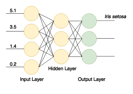
After successful training, we’ll have a network that receives four values via its inputs and sends a signal to one of its three outputs. This is a simple classifier.
Finally, to finish building the network, we set up back propagation (one of the most effective training methods) and disable pre-training with the line .backprop(true).pretrain(false).
6. Creating and Training a Network
Now let’s create a neural network from the configuration, initialize and run it:
MultiLayerNetwork model = new MultiLayerNetwork(configuration);
model.init();
model.fit(trainingData);
Now we can test the trained model by using the rest of the dataset and verify the results with evaluation metrics for three classes:
INDArray output = model.output(testData.getFeatureMatrix());
Evaluation eval = new Evaluation(3);
eval.eval(testData.getLabels(), output);
If we now print out the eval.stats(), we’ll see that our network is pretty good at classifying iris flowers, although it did mistake class 1 for class 2 three times.
Examples labeled as 0 classified by model as 0: 19 times
Examples labeled as 1 classified by model as 1: 16 times
Examples labeled as 1 classified by model as 2: 3 times
Examples labeled as 2 classified by model as 2: 15 times

==========================Scores========================================
# of classes: 3
Accuracy: 0.9434
Precision: 0.9444
Recall: 0.9474
F1 Score: 0.9411
Precision, recall & F1: macro-averaged (equally weighted avg. of 3 classes)
========================================================================
The fluent configuration builder allows us to add or modify layers of the network quickly, or tweak some other parameters to see if our model can be improved.
7. Conclusion
In this article, we’ve built a simple yet powerful neural network by using the deeplearning4j library.